模型构建

《区域水环境污染数据分析实践》
Data analysis practice of regional water environment pollution

苏命、王为东
中国科学院大学资源与环境学院
中国科学院生态环境研究中心

2025-04-09

大纲

• tidymodels主要步骤
• 实践部分

tidymodels主要步骤

何为tidymodels?

library(tidymodels)

#> ── Attaching packages ──────────────────────────── tidymodels 1.2.0 ──

#> ✔ broom        1.0.7     ✔ rsample      1.2.1
#> ✔ dials        1.4.0     ✔ tibble       3.2.1
#> ✔ dplyr        1.1.4     ✔ tidyr        1.3.1
#> ✔ infer        1.0.7     ✔ tune         1.2.1
#> ✔ modeldata    1.4.0     ✔ workflows    1.1.4
#> ✔ parsnip      1.2.1     ✔ workflowsets 1.1.0
#> ✔ purrr        1.0.4     ✔ yardstick    1.3.2
#> ✔ recipes      1.1.0

#> ── Conflicts ─────────────────────────────── tidymodels_conflicts() ──
#> ✖ purrr::discard() masks scales::discard()
#> ✖ dplyr::filter()  masks stats::filter()
#> ✖ dplyr::lag()     masks stats::lag()
#> ✖ recipes::step()  masks stats::step()
#> • Use suppressPackageStartupMessages() to eliminate package startup messages

整体思路

整体思路

Stress that we are not fitting a model on the entire training set other than for illustrative purposes in deck 2.

整体思路

整体思路

整体思路

整体思路

整体思路

相关包的安装

# Install the packages for the workshop
pkgs <-
  c(
    "bonsai",
    "doParallel",
    "embed",
    "finetune",
    "lightgbm",
    "lme4",
    "plumber",
    "probably",
    "ranger",
    "rpart",
    "rpart.plot",
    "rules",
    "splines2",
    "stacks",
    "text2vec",
    "textrecipes",
    "tidymodels",
    "vetiver",
    "remotes"
  )

install.packages(pkgs)

Data on Chicago taxi trips

library(tidymodels)
taxi

#> # A tibble: 10,000 × 7
#>    tip   distance company                      local dow   month  hour
#>    <fct>    <dbl> <fct>                        <fct> <fct> <fct> <int>
#>  1 yes      17.2  Chicago Independents         no    Thu   Feb      16
#>  2 yes       0.88 City Service                 yes   Thu   Mar       8
#>  3 yes      18.1  other                        no    Mon   Feb      18
#>  4 yes      20.7  Chicago Independents         no    Mon   Apr       8
#>  5 yes      12.2  Chicago Independents         no    Sun   Mar      21
#>  6 yes       0.94 Sun Taxi                     yes   Sat   Apr      23
#>  7 yes      17.5  Flash Cab                    no    Fri   Mar      12
#>  8 yes      17.7  other                        no    Sun   Jan       6
#>  9 yes       1.85 Taxicab Insurance Agency Llc no    Fri   Apr      12
#> 10 yes       1.47 City Service                 no    Tue   Mar      14
#> # ℹ 9,990 more rows

数据分割与使用

对于机器学习，我们通常将数据分成训练集和测试集：

• 训练集用于估计模型参数。
• 测试集用于独立评估模型性能。

在训练过程中不要使用测试集。

The initial split

set.seed(123)
taxi_split <- initial_split(taxi)
taxi_split

#> <Training/Testing/Total>
#> <7500/2500/10000>

Accessing the data

taxi_train <- training(taxi_split)
taxi_test <- testing(taxi_split)

The training set

taxi_train

#> # A tibble: 7,500 × 7
#>    tip   distance company                   local dow   month  hour
#>    <fct>    <dbl> <fct>                     <fct> <fct> <fct> <int>
#>  1 yes       0.7  Taxi Affiliation Services yes   Tue   Mar      18
#>  2 yes       0.99 Sun Taxi                  yes   Tue   Jan       8
#>  3 yes       1.78 other                     no    Sat   Mar      22
#>  4 yes       0    Taxi Affiliation Services yes   Wed   Apr      15
#>  5 yes       0    Taxi Affiliation Services no    Sun   Jan      21
#>  6 yes       2.3  other                     no    Sat   Apr      21
#>  7 yes       6.35 Sun Taxi                  no    Wed   Mar      16
#>  8 yes       2.79 other                     no    Sun   Feb      14
#>  9 yes      16.6  other                     no    Sun   Apr      18
#> 10 yes       0.02 Chicago Independents      yes   Sun   Apr      15
#> # ℹ 7,490 more rows

练习

set.seed(123)
taxi_split <- initial_split(taxi, prop = 0.8)
taxi_train <- training(taxi_split)
taxi_test <- testing(taxi_split)

nrow(taxi_train)

#> [1] 8000

nrow(taxi_test)

#> [1] 2000

Stratification

Use strata = tip

set.seed(123)
taxi_split <- initial_split(taxi, prop = 0.8, strata = tip)
taxi_split

#> <Training/Testing/Total>
#> <8000/2000/10000>

Stratification

Stratification often helps, with very little downside

模型类型

模型多种多样

• lm for linear model

• glm for generalized linear model (e.g. logistic regression)

• glmnet for regularized regression

• keras for regression using TensorFlow

• stan for Bayesian regression

• spark for large data sets

指定模型

logistic_reg()

#> Logistic Regression Model Specification (classification)
#> 
#> Computational engine: glm

Models have default engines

To specify a model

logistic_reg() %>%
  set_engine("glmnet")

#> Logistic Regression Model Specification (classification)
#> 
#> Computational engine: glmnet

logistic_reg() %>%
  set_engine("stan")

#> Logistic Regression Model Specification (classification)
#> 
#> Computational engine: stan

• Choose a model
• Specify an engine
• Set the mode

To specify a model

decision_tree()

#> Decision Tree Model Specification (unknown mode)
#> 
#> Computational engine: rpart

Some models have a default mode

To specify a model

decision_tree() %>%
  set_mode("classification")

#> Decision Tree Model Specification (classification)
#> 
#> Computational engine: rpart

All available models are listed at https://www.tidymodels.org/find/parsnip/

Workflows

为什么要使用 workflow()?

• 与基本的 R 工具相比，工作流能更好地处理新的因子水平

• 除了公式之外，还可以使用其他的预处理器（更多关于高级 tidymodels 中的特征工程！）

• 在使用多个模型时，它们可以帮助组织工作

• 最重要的是，工作流涵盖了整个建模过程：fit() 和 predict() 不仅适用于实际的模型拟合，还适用于预处理步骤

工作流比基本的 R 处理水平更好的两种方式：

• 强制要求在预测时不允许出现新的水平（这是一个可选的检查，可以关闭）

• 恢复在拟合时存在但在预测时缺失的水平（例如，“新”数据中没有该水平的实例）

A model workflow

tree_spec <-
  decision_tree(cost_complexity = 0.002) %>%
  set_mode("classification")

tree_spec %>%
  fit(tip ~ ., data = taxi_train)

#> parsnip model object
#> 
#> n= 8000 
#> 
#> node), split, n, loss, yval, (yprob)
#>       * denotes terminal node
#> 
#>  1) root 8000 616 yes (0.92300000 0.07700000)  
#>    2) distance>=14.12 2041  68 yes (0.96668300 0.03331700) *
#>    3) distance< 14.12 5959 548 yes (0.90803826 0.09196174)  
#>      6) distance< 5.275 5419 450 yes (0.91695885 0.08304115) *
#>      7) distance>=5.275 540  98 yes (0.81851852 0.18148148)  
#>       14) company=Chicago Independents,City Service,Sun Taxi,Taxi Affiliation Services,Taxicab Insurance Agency Llc,other 478  68 yes (0.85774059 0.14225941) *
#>       15) company=Flash Cab 62  30 yes (0.51612903 0.48387097)  
#>         30) dow=Thu 12   2 yes (0.83333333 0.16666667) *
#>         31) dow=Sun,Mon,Tue,Wed,Fri,Sat 50  22 no (0.44000000 0.56000000)  
#>           62) distance>=11.77 14   4 yes (0.71428571 0.28571429) *
#>           63) distance< 11.77 36  12 no (0.33333333 0.66666667) *

A model workflow

tree_spec <-
  decision_tree(cost_complexity = 0.002) %>%
  set_mode("classification")

workflow() %>%
  add_formula(tip ~ .) %>%
  add_model(tree_spec) %>%
  fit(data = taxi_train)

#> ══ Workflow [trained] ════════════════════════════════════════════════
#> Preprocessor: Formula
#> Model: decision_tree()
#> 
#> ── Preprocessor ──────────────────────────────────────────────────────
#> tip ~ .
#> 
#> ── Model ─────────────────────────────────────────────────────────────
#> n= 8000 
#> 
#> node), split, n, loss, yval, (yprob)
#>       * denotes terminal node
#> 
#>  1) root 8000 616 yes (0.92300000 0.07700000)  
#>    2) distance>=14.12 2041  68 yes (0.96668300 0.03331700) *
#>    3) distance< 14.12 5959 548 yes (0.90803826 0.09196174)  
#>      6) distance< 5.275 5419 450 yes (0.91695885 0.08304115) *
#>      7) distance>=5.275 540  98 yes (0.81851852 0.18148148)  
#>       14) company=Chicago Independents,City Service,Sun Taxi,Taxi Affiliation Services,Taxicab Insurance Agency Llc,other 478  68 yes (0.85774059 0.14225941) *
#>       15) company=Flash Cab 62  30 yes (0.51612903 0.48387097)  
#>         30) dow=Thu 12   2 yes (0.83333333 0.16666667) *
#>         31) dow=Sun,Mon,Tue,Wed,Fri,Sat 50  22 no (0.44000000 0.56000000)  
#>           62) distance>=11.77 14   4 yes (0.71428571 0.28571429) *
#>           63) distance< 11.77 36  12 no (0.33333333 0.66666667) *

A model workflow

tree_spec <-
  decision_tree(cost_complexity = 0.002) %>%
  set_mode("classification")

workflow(tip ~ ., tree_spec) %>%
  fit(data = taxi_train)

#> ══ Workflow [trained] ════════════════════════════════════════════════
#> Preprocessor: Formula
#> Model: decision_tree()
#> 
#> ── Preprocessor ──────────────────────────────────────────────────────
#> tip ~ .
#> 
#> ── Model ─────────────────────────────────────────────────────────────
#> n= 8000 
#> 
#> node), split, n, loss, yval, (yprob)
#>       * denotes terminal node
#> 
#>  1) root 8000 616 yes (0.92300000 0.07700000)  
#>    2) distance>=14.12 2041  68 yes (0.96668300 0.03331700) *
#>    3) distance< 14.12 5959 548 yes (0.90803826 0.09196174)  
#>      6) distance< 5.275 5419 450 yes (0.91695885 0.08304115) *
#>      7) distance>=5.275 540  98 yes (0.81851852 0.18148148)  
#>       14) company=Chicago Independents,City Service,Sun Taxi,Taxi Affiliation Services,Taxicab Insurance Agency Llc,other 478  68 yes (0.85774059 0.14225941) *
#>       15) company=Flash Cab 62  30 yes (0.51612903 0.48387097)  
#>         30) dow=Thu 12   2 yes (0.83333333 0.16666667) *
#>         31) dow=Sun,Mon,Tue,Wed,Fri,Sat 50  22 no (0.44000000 0.56000000)  
#>           62) distance>=11.77 14   4 yes (0.71428571 0.28571429) *
#>           63) distance< 11.77 36  12 no (0.33333333 0.66666667) *

预测

How do you use your new tree_fit model?

tree_spec <-
  decision_tree(cost_complexity = 0.002) %>%
  set_mode("classification")

tree_fit <-
  workflow(tip ~ ., tree_spec) %>%
  fit(data = taxi_train)

练习

Run:

predict(tree_fit, new_data = taxi_test)

Run:

augment(tree_fit, new_data = taxi_test)

What do you get?

tidymodels 的预测

• 预测结果始终在一个 tibble 内
• 列名和类型可读性强
• new_data 中的行数和输出中的行数相同

理解模型

如何 理解tree_fit 模型？

Evaluating models: 预测值

augment(taxi_fit, new_data = taxi_train) %>%
  relocate(tip, .pred_class, .pred_yes, .pred_no)

#> # A tibble: 8,000 × 10
#>    tip   .pred_class .pred_yes .pred_no distance company local dow   month  hour
#>    <fct> <fct>           <dbl>    <dbl>    <dbl> <fct>   <fct> <fct> <fct> <int>
#>  1 yes   yes             0.967   0.0333    17.2  Chicag… no    Thu   Feb      16
#>  2 yes   yes             0.935   0.0646     0.88 City S… yes   Thu   Mar       8
#>  3 yes   yes             0.967   0.0333    18.1  other   no    Mon   Feb      18
#>  4 yes   yes             0.949   0.0507    12.2  Chicag… no    Sun   Mar      21
#>  5 yes   yes             0.821   0.179      0.94 Sun Ta… yes   Sat   Apr      23
#>  6 yes   yes             0.967   0.0333    17.5  Flash … no    Fri   Mar      12
#>  7 yes   yes             0.967   0.0333    17.7  other   no    Sun   Jan       6
#>  8 yes   yes             0.938   0.0616     1.85 Taxica… no    Fri   Apr      12
#>  9 yes   yes             0.938   0.0616     0.53 Sun Ta… no    Tue   Mar      18
#> 10 yes   yes             0.931   0.0694     6.65 Taxica… no    Sun   Apr      11
#> # ℹ 7,990 more rows

Confusion matrix

Confusion matrix

augment(taxi_fit, new_data = taxi_train) %>%
  conf_mat(truth = tip, estimate = .pred_class)

#>           Truth
#> Prediction  yes   no
#>        yes 7341  536
#>        no    43   80

Confusion matrix

augment(taxi_fit, new_data = taxi_train) %>%
  conf_mat(truth = tip, estimate = .pred_class) %>%
  autoplot(type = "heatmap")

Metrics for model performance

augment(taxi_fit, new_data = taxi_train) %>%
  accuracy(truth = tip, estimate = .pred_class)

#> # A tibble: 1 × 3
#>   .metric  .estimator .estimate
#>   <chr>    <chr>          <dbl>
#> 1 accuracy binary         0.928

二分类模型评估

模型的敏感性（Sensitivity）和特异性（Specificity）是评估二分类模型性能的重要指标：

• 敏感性（Sensitivity），也称为真阳性率，衡量了模型正确识别正类别样本的能力。公式为真阳性数除以真阳性数加上假阴性数：

\[ \text{Sensitivity} = \frac{\text{True Positives}}{\text{True Positives} + \text{False Negatives}} \]

• 特异性（Specificity），也称为真阴性率，衡量了模型正确识别负类别样本的能力。公式为真阴性数除以真阴性数加上假阳性数：

\[ \text{Specificity} = \frac{\text{True Negatives}}{\text{True Negatives} + \text{False Positives}} \]

在评估模型时，我们希望敏感性和特异性都很高。高敏感性表示模型能够捕获真正的正类别样本，高特异性表示模型能够准确排除负类别样本。

Metrics for model performance

augment(taxi_fit, new_data = taxi_train) %>%
  sensitivity(truth = tip, estimate = .pred_class)

#> # A tibble: 1 × 3
#>   .metric     .estimator .estimate
#>   <chr>       <chr>          <dbl>
#> 1 sensitivity binary         0.994

Metrics for model performance

augment(taxi_fit, new_data = taxi_train) %>%
  sensitivity(truth = tip, estimate = .pred_class)

#> # A tibble: 1 × 3
#>   .metric     .estimator .estimate
#>   <chr>       <chr>          <dbl>
#> 1 sensitivity binary         0.994

augment(taxi_fit, new_data = taxi_train) %>%
  specificity(truth = tip, estimate = .pred_class)

#> # A tibble: 1 × 3
#>   .metric     .estimator .estimate
#>   <chr>       <chr>          <dbl>
#> 1 specificity binary         0.130

Metrics for model performance

We can use metric_set() to combine multiple calculations into one

taxi_metrics <- metric_set(accuracy, specificity, sensitivity)

augment(taxi_fit, new_data = taxi_train) %>%
  taxi_metrics(truth = tip, estimate = .pred_class)

#> # A tibble: 3 × 3
#>   .metric     .estimator .estimate
#>   <chr>       <chr>          <dbl>
#> 1 accuracy    binary         0.928
#> 2 specificity binary         0.130
#> 3 sensitivity binary         0.994

Metrics for model performance

taxi_metrics <- metric_set(accuracy, specificity, sensitivity)

augment(taxi_fit, new_data = taxi_train) %>%
  group_by(local) %>%
  taxi_metrics(truth = tip, estimate = .pred_class)

#> # A tibble: 6 × 4
#>   local .metric     .estimator .estimate
#>   <fct> <chr>       <chr>          <dbl>
#> 1 yes   accuracy    binary         0.898
#> 2 no    accuracy    binary         0.935
#> 3 yes   specificity binary         0.169
#> 4 no    specificity binary         0.116
#> 5 yes   sensitivity binary         0.987
#> 6 no    sensitivity binary         0.996

Varying the threshold

ROC 曲线

• ROC（Receiver Operating Characteristic）曲线用于评估二分类模型的性能，特别是在不同的阈值下比较模型的敏感性和特异性。
• ROC曲线的横轴是假阳性率（False Positive Rate，FPR），纵轴是真阳性率（True Positive Rate，TPR）。在ROC曲线上，每个点对应于一个特定的阈值。通过改变阈值，我们可以观察到模型在不同条件下的表现。
• ROC曲线越接近左上角（0,1）点，说明模型的性能越好，因为这表示在较低的假阳性率下，模型能够获得较高的真阳性率。ROC曲线下面积（Area Under the ROC Curve，AUC）也是评估模型性能的一种指标，AUC值越大表示模型性能越好。

ROC curve plot

augment(taxi_fit, new_data = taxi_train) %>%
  roc_curve(truth = tip, .pred_yes) %>%
  autoplot()

过度拟合

过度拟合

Cross-validation

Cross-validation

Cross-validation

Cross-validation

vfold_cv(taxi_train) # v = 10 is default

#> #  10-fold cross-validation 
#> # A tibble: 10 × 2
#>    splits             id    
#>    <list>             <chr> 
#>  1 <split [7200/800]> Fold01
#>  2 <split [7200/800]> Fold02
#>  3 <split [7200/800]> Fold03
#>  4 <split [7200/800]> Fold04
#>  5 <split [7200/800]> Fold05
#>  6 <split [7200/800]> Fold06
#>  7 <split [7200/800]> Fold07
#>  8 <split [7200/800]> Fold08
#>  9 <split [7200/800]> Fold09
#> 10 <split [7200/800]> Fold10

Cross-validation

What is in this?

taxi_folds <- vfold_cv(taxi_train)
taxi_folds$splits[1:3]

#> [[1]]
#> <Analysis/Assess/Total>
#> <7200/800/8000>
#> 
#> [[2]]
#> <Analysis/Assess/Total>
#> <7200/800/8000>
#> 
#> [[3]]
#> <Analysis/Assess/Total>
#> <7200/800/8000>

Talk about a list column, storing non-atomic types in dataframe

Cross-validation

vfold_cv(taxi_train, v = 5)

#> #  5-fold cross-validation 
#> # A tibble: 5 × 2
#>   splits              id   
#>   <list>              <chr>
#> 1 <split [6400/1600]> Fold1
#> 2 <split [6400/1600]> Fold2
#> 3 <split [6400/1600]> Fold3
#> 4 <split [6400/1600]> Fold4
#> 5 <split [6400/1600]> Fold5

Cross-validation

vfold_cv(taxi_train, strata = tip)

#> #  10-fold cross-validation using stratification 
#> # A tibble: 10 × 2
#>    splits             id    
#>    <list>             <chr> 
#>  1 <split [7200/800]> Fold01
#>  2 <split [7200/800]> Fold02
#>  3 <split [7200/800]> Fold03
#>  4 <split [7200/800]> Fold04
#>  5 <split [7200/800]> Fold05
#>  6 <split [7200/800]> Fold06
#>  7 <split [7200/800]> Fold07
#>  8 <split [7200/800]> Fold08
#>  9 <split [7200/800]> Fold09
#> 10 <split [7200/800]> Fold10

Stratification often helps, with very little downside

Cross-validation

We’ll use this setup:

set.seed(123)
taxi_folds <- vfold_cv(taxi_train, v = 10, strata = tip)
taxi_folds

#> #  10-fold cross-validation using stratification 
#> # A tibble: 10 × 2
#>    splits             id    
#>    <list>             <chr> 
#>  1 <split [7200/800]> Fold01
#>  2 <split [7200/800]> Fold02
#>  3 <split [7200/800]> Fold03
#>  4 <split [7200/800]> Fold04
#>  5 <split [7200/800]> Fold05
#>  6 <split [7200/800]> Fold06
#>  7 <split [7200/800]> Fold07
#>  8 <split [7200/800]> Fold08
#>  9 <split [7200/800]> Fold09
#> 10 <split [7200/800]> Fold10

Set the seed when creating resamples

Fit our model to the resamples

taxi_res <- fit_resamples(taxi_wflow, taxi_folds)
taxi_res

#> # Resampling results
#> # 10-fold cross-validation using stratification 
#> # A tibble: 10 × 4
#>    splits             id     .metrics         .notes          
#>    <list>             <chr>  <list>           <list>          
#>  1 <split [7200/800]> Fold01 <tibble [3 × 4]> <tibble [0 × 3]>
#>  2 <split [7200/800]> Fold02 <tibble [3 × 4]> <tibble [0 × 3]>
#>  3 <split [7200/800]> Fold03 <tibble [3 × 4]> <tibble [0 × 3]>
#>  4 <split [7200/800]> Fold04 <tibble [3 × 4]> <tibble [0 × 3]>
#>  5 <split [7200/800]> Fold05 <tibble [3 × 4]> <tibble [0 × 3]>
#>  6 <split [7200/800]> Fold06 <tibble [3 × 4]> <tibble [0 × 3]>
#>  7 <split [7200/800]> Fold07 <tibble [3 × 4]> <tibble [0 × 3]>
#>  8 <split [7200/800]> Fold08 <tibble [3 × 4]> <tibble [0 × 3]>
#>  9 <split [7200/800]> Fold09 <tibble [3 × 4]> <tibble [0 × 3]>
#> 10 <split [7200/800]> Fold10 <tibble [3 × 4]> <tibble [0 × 3]>

Evaluating model performance

taxi_res %>%
  collect_metrics()

#> # A tibble: 3 × 6
#>   .metric     .estimator   mean     n std_err .config             
#>   <chr>       <chr>       <dbl> <int>   <dbl> <chr>               
#> 1 accuracy    binary     0.915     10 0.00309 Preprocessor1_Model1
#> 2 brier_class binary     0.0721    10 0.00245 Preprocessor1_Model1
#> 3 roc_auc     binary     0.624     10 0.0105  Preprocessor1_Model1

collect_metrics() 是一套 collect_() 函数之一，可用于处理调参结果的列。调参结果中以 . 为前缀的大多数列都有对应的 collect_() 函数，可以进行常见摘要选项的汇总。

We can reliably measure performance using only the training data 🎉

Comparing metrics

How do the metrics from resampling compare to the metrics from training and testing?

taxi_res %>%
  collect_metrics() %>%
  select(.metric, mean, n)

#> # A tibble: 3 × 3
#>   .metric       mean     n
#>   <chr>        <dbl> <int>
#> 1 accuracy    0.915     10
#> 2 brier_class 0.0721    10
#> 3 roc_auc     0.624     10

The ROC AUC previously was

• 0.69 for the training set
• 0.64 for test set

Remember that:

⚠️ the training set gives you overly optimistic metrics

⚠️ the test set is precious

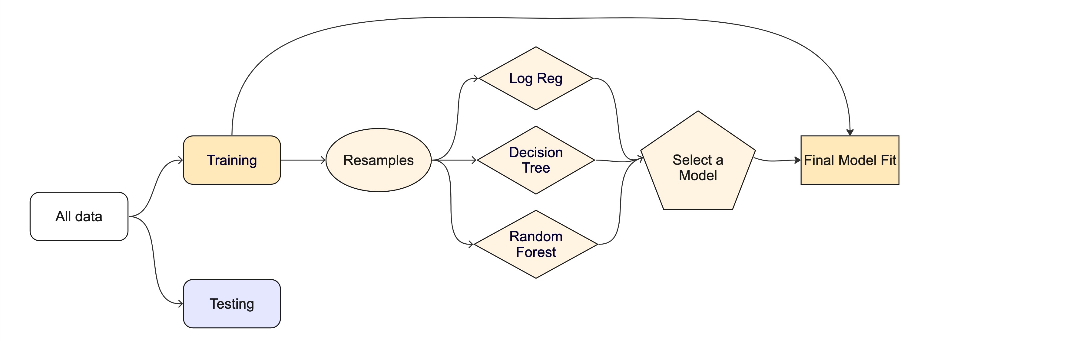
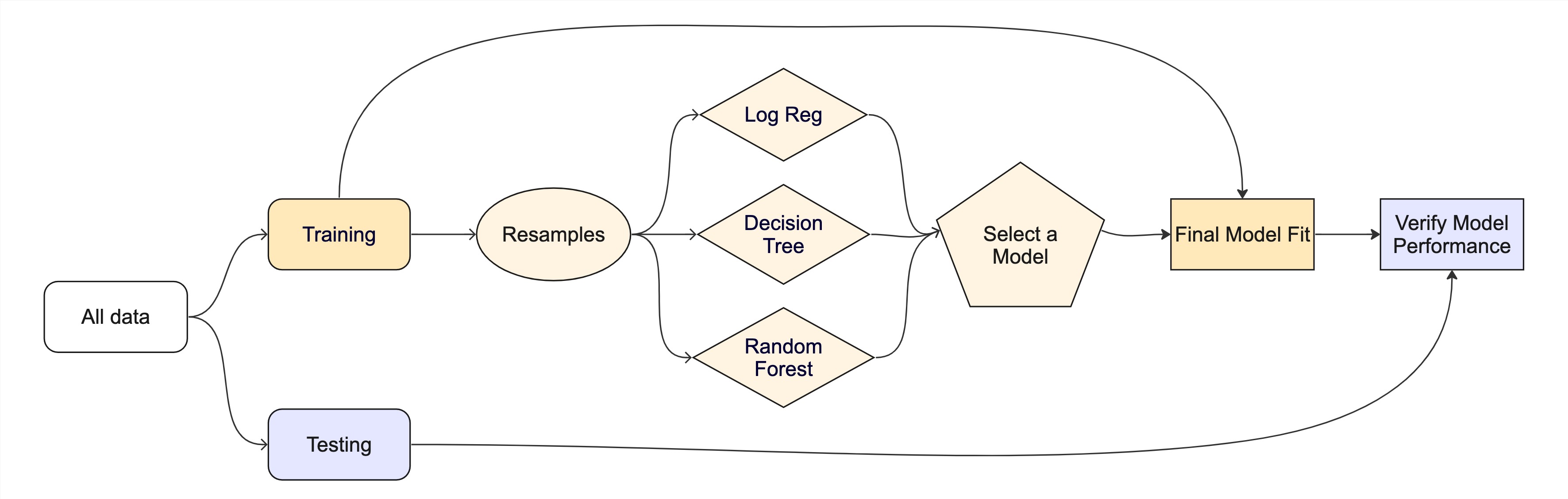
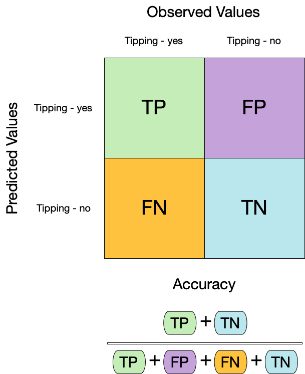
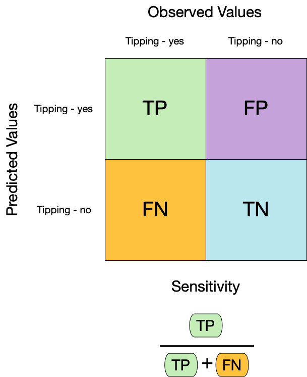
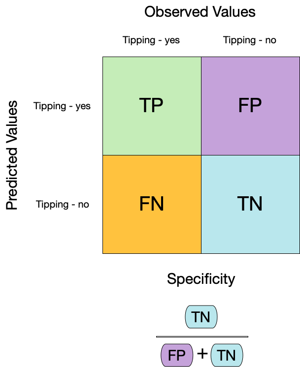
Evaluating model performance

# Save the assessment set results
ctrl_taxi <- control_resamples(save_pred = TRUE)
taxi_res <- fit_resamples(taxi_wflow, taxi_folds, control = ctrl_taxi)

taxi_res

#> # Resampling results
#> # 10-fold cross-validation using stratification 
#> # A tibble: 10 × 5
#>    splits             id     .metrics         .notes           .predictions
#>    <list>             <chr>  <list>           <list>           <list>      
#>  1 <split [7200/800]> Fold01 <tibble [3 × 4]> <tibble [0 × 3]> <tibble>    
#>  2 <split [7200/800]> Fold02 <tibble [3 × 4]> <tibble [0 × 3]> <tibble>    
#>  3 <split [7200/800]> Fold03 <tibble [3 × 4]> <tibble [0 × 3]> <tibble>    
#>  4 <split [7200/800]> Fold04 <tibble [3 × 4]> <tibble [0 × 3]> <tibble>    
#>  5 <split [7200/800]> Fold05 <tibble [3 × 4]> <tibble [0 × 3]> <tibble>    
#>  6 <split [7200/800]> Fold06 <tibble [3 × 4]> <tibble [0 × 3]> <tibble>    
#>  7 <split [7200/800]> Fold07 <tibble [3 × 4]> <tibble [0 × 3]> <tibble>    
#>  8 <split [7200/800]> Fold08 <tibble [3 × 4]> <tibble [0 × 3]> <tibble>    
#>  9 <split [7200/800]> Fold09 <tibble [3 × 4]> <tibble [0 × 3]> <tibble>    
#> 10 <split [7200/800]> Fold10 <tibble [3 × 4]> <tibble [0 × 3]> <tibble>

Evaluating model performance

# Save the assessment set results
taxi_preds <- collect_predictions(taxi_res)
taxi_preds

#> # A tibble: 8,000 × 7
#>    .pred_class .pred_yes .pred_no id      .row tip   .config             
#>    <fct>           <dbl>    <dbl> <chr>  <int> <fct> <chr>               
#>  1 yes             0.938   0.0615 Fold01    14 yes   Preprocessor1_Model1
#>  2 yes             0.946   0.0544 Fold01    19 yes   Preprocessor1_Model1
#>  3 yes             0.973   0.0269 Fold01    33 yes   Preprocessor1_Model1
#>  4 yes             0.903   0.0971 Fold01    43 yes   Preprocessor1_Model1
#>  5 yes             0.973   0.0269 Fold01    74 yes   Preprocessor1_Model1
#>  6 yes             0.903   0.0971 Fold01   103 yes   Preprocessor1_Model1
#>  7 yes             0.915   0.0851 Fold01   104 no    Preprocessor1_Model1
#>  8 yes             0.903   0.0971 Fold01   124 yes   Preprocessor1_Model1
#>  9 yes             0.667   0.333  Fold01   126 yes   Preprocessor1_Model1
#> 10 yes             0.949   0.0510 Fold01   128 yes   Preprocessor1_Model1
#> # ℹ 7,990 more rows

Evaluating model performance

taxi_preds %>%
  group_by(id) %>%
  taxi_metrics(truth = tip, estimate = .pred_class)

#> # A tibble: 30 × 4
#>    id     .metric  .estimator .estimate
#>    <chr>  <chr>    <chr>          <dbl>
#>  1 Fold01 accuracy binary         0.905
#>  2 Fold02 accuracy binary         0.925
#>  3 Fold03 accuracy binary         0.926
#>  4 Fold04 accuracy binary         0.915
#>  5 Fold05 accuracy binary         0.902
#>  6 Fold06 accuracy binary         0.912
#>  7 Fold07 accuracy binary         0.906
#>  8 Fold08 accuracy binary         0.91 
#>  9 Fold09 accuracy binary         0.918
#> 10 Fold10 accuracy binary         0.931
#> # ℹ 20 more rows

Where are the fitted models?

taxi_res

#> # Resampling results
#> # 10-fold cross-validation using stratification 
#> # A tibble: 10 × 5
#>    splits             id     .metrics         .notes           .predictions
#>    <list>             <chr>  <list>           <list>           <list>      
#>  1 <split [7200/800]> Fold01 <tibble [3 × 4]> <tibble [0 × 3]> <tibble>    
#>  2 <split [7200/800]> Fold02 <tibble [3 × 4]> <tibble [0 × 3]> <tibble>    
#>  3 <split [7200/800]> Fold03 <tibble [3 × 4]> <tibble [0 × 3]> <tibble>    
#>  4 <split [7200/800]> Fold04 <tibble [3 × 4]> <tibble [0 × 3]> <tibble>    
#>  5 <split [7200/800]> Fold05 <tibble [3 × 4]> <tibble [0 × 3]> <tibble>    
#>  6 <split [7200/800]> Fold06 <tibble [3 × 4]> <tibble [0 × 3]> <tibble>    
#>  7 <split [7200/800]> Fold07 <tibble [3 × 4]> <tibble [0 × 3]> <tibble>    
#>  8 <split [7200/800]> Fold08 <tibble [3 × 4]> <tibble [0 × 3]> <tibble>    
#>  9 <split [7200/800]> Fold09 <tibble [3 × 4]> <tibble [0 × 3]> <tibble>    
#> 10 <split [7200/800]> Fold10 <tibble [3 × 4]> <tibble [0 × 3]> <tibble>

Bootstrapping

Bootstrapping

set.seed(3214)
bootstraps(taxi_train)

#> # Bootstrap sampling 
#> # A tibble: 25 × 2
#>    splits              id         
#>    <list>              <chr>      
#>  1 <split [8000/2902]> Bootstrap01
#>  2 <split [8000/2916]> Bootstrap02
#>  3 <split [8000/3004]> Bootstrap03
#>  4 <split [8000/2979]> Bootstrap04
#>  5 <split [8000/2961]> Bootstrap05
#>  6 <split [8000/2962]> Bootstrap06
#>  7 <split [8000/3026]> Bootstrap07
#>  8 <split [8000/2926]> Bootstrap08
#>  9 <split [8000/2972]> Bootstrap09
#> 10 <split [8000/2972]> Bootstrap10
#> # ℹ 15 more rows

Monte Carlo Cross-Validation

set.seed(322)
mc_cv(taxi_train, times = 10)

#> # Monte Carlo cross-validation (0.75/0.25) with 10 resamples  
#> # A tibble: 10 × 2
#>    splits              id        
#>    <list>              <chr>     
#>  1 <split [6000/2000]> Resample01
#>  2 <split [6000/2000]> Resample02
#>  3 <split [6000/2000]> Resample03
#>  4 <split [6000/2000]> Resample04
#>  5 <split [6000/2000]> Resample05
#>  6 <split [6000/2000]> Resample06
#>  7 <split [6000/2000]> Resample07
#>  8 <split [6000/2000]> Resample08
#>  9 <split [6000/2000]> Resample09
#> 10 <split [6000/2000]> Resample10

Validation set

set.seed(853)
taxi_val_split <- initial_validation_split(taxi, strata = tip)
validation_set(taxi_val_split)

#> # A tibble: 1 × 2
#>   splits              id        
#>   <list>              <chr>     
#> 1 <split [6000/2000]> validation

Create a random forest model

rf_spec <- rand_forest(trees = 1000, mode = "classification")
rf_spec

#> Random Forest Model Specification (classification)
#> 
#> Main Arguments:
#>   trees = 1000
#> 
#> Computational engine: ranger

Create a random forest model

rf_wflow <- workflow(tip ~ ., rf_spec)
rf_wflow

#> ══ Workflow ══════════════════════════════════════════════════════════
#> Preprocessor: Formula
#> Model: rand_forest()
#> 
#> ── Preprocessor ──────────────────────────────────────────────────────
#> tip ~ .
#> 
#> ── Model ─────────────────────────────────────────────────────────────
#> Random Forest Model Specification (classification)
#> 
#> Main Arguments:
#>   trees = 1000
#> 
#> Computational engine: ranger

Evaluating model performance

ctrl_taxi <- control_resamples(save_pred = TRUE)

# Random forest uses random numbers so set the seed first

set.seed(2)
rf_res <- fit_resamples(rf_wflow, taxi_folds, control = ctrl_taxi)
collect_metrics(rf_res)

#> # A tibble: 3 × 6
#>   .metric     .estimator   mean     n std_err .config             
#>   <chr>       <chr>       <dbl> <int>   <dbl> <chr>               
#> 1 accuracy    binary     0.923     10 0.00317 Preprocessor1_Model1
#> 2 brier_class binary     0.0706    10 0.00243 Preprocessor1_Model1
#> 3 roc_auc     binary     0.616     10 0.0147  Preprocessor1_Model1

The whole game - status update

The final fit

# taxi_split has train + test info
final_fit <- last_fit(rf_wflow, taxi_split)

final_fit

#> # Resampling results
#> # Manual resampling 
#> # A tibble: 1 × 6
#>   splits              id               .metrics .notes   .predictions .workflow 
#>   <list>              <chr>            <list>   <list>   <list>       <list>    
#> 1 <split [8000/2000]> train/test split <tibble> <tibble> <tibble>     <workflow>

何为final_fit?

collect_metrics(final_fit)

#> # A tibble: 3 × 4
#>   .metric     .estimator .estimate .config             
#>   <chr>       <chr>          <dbl> <chr>               
#> 1 accuracy    binary        0.914  Preprocessor1_Model1
#> 2 roc_auc     binary        0.638  Preprocessor1_Model1
#> 3 brier_class binary        0.0772 Preprocessor1_Model1

These are metrics computed with the test set

何为final_fit?

collect_predictions(final_fit)

#> # A tibble: 2,000 × 7
#>    .pred_class .pred_yes .pred_no id                .row tip   .config          
#>    <fct>           <dbl>    <dbl> <chr>            <int> <fct> <chr>            
#>  1 yes             0.957   0.0426 train/test split     4 yes   Preprocessor1_Mo…
#>  2 yes             0.938   0.0621 train/test split    10 yes   Preprocessor1_Mo…
#>  3 yes             0.958   0.0416 train/test split    19 yes   Preprocessor1_Mo…
#>  4 yes             0.894   0.106  train/test split    23 yes   Preprocessor1_Mo…
#>  5 yes             0.943   0.0573 train/test split    28 yes   Preprocessor1_Mo…
#>  6 yes             0.979   0.0213 train/test split    34 yes   Preprocessor1_Mo…
#>  7 yes             0.954   0.0463 train/test split    35 yes   Preprocessor1_Mo…
#>  8 yes             0.928   0.0722 train/test split    38 yes   Preprocessor1_Mo…
#>  9 yes             0.985   0.0147 train/test split    40 yes   Preprocessor1_Mo…
#> 10 yes             0.948   0.0523 train/test split    42 no    Preprocessor1_Mo…
#> # ℹ 1,990 more rows

何为final_fit?

extract_workflow(final_fit)

#> ══ Workflow [trained] ════════════════════════════════════════════════
#> Preprocessor: Formula
#> Model: rand_forest()
#> 
#> ── Preprocessor ──────────────────────────────────────────────────────
#> tip ~ .
#> 
#> ── Model ─────────────────────────────────────────────────────────────
#> Ranger result
#> 
#> Call:
#>  ranger::ranger(x = maybe_data_frame(x), y = y, num.trees = ~1000,      num.threads = 1, verbose = FALSE, seed = sample.int(10^5,          1), probability = TRUE) 
#> 
#> Type:                             Probability estimation 
#> Number of trees:                  1000 
#> Sample size:                      8000 
#> Number of independent variables:  6 
#> Mtry:                             2 
#> Target node size:                 10 
#> Variable importance mode:         none 
#> Splitrule:                        gini 
#> OOB prediction error (Brier s.):  0.07069778

Use this for prediction on new data, like for deploying

Tuning models - Specifying tuning parameters

rf_spec <- rand_forest(min_n = tune()) %>%
  set_mode("classification")

rf_wflow <- workflow(tip ~ ., rf_spec)
rf_wflow

#> ══ Workflow ══════════════════════════════════════════════════════════
#> Preprocessor: Formula
#> Model: rand_forest()
#> 
#> ── Preprocessor ──────────────────────────────────────────────────────
#> tip ~ .
#> 
#> ── Model ─────────────────────────────────────────────────────────────
#> Random Forest Model Specification (classification)
#> 
#> Main Arguments:
#>   min_n = tune()
#> 
#> Computational engine: ranger

Try out multiple values

tune_grid() works similar to fit_resamples() but covers multiple parameter values:

set.seed(22)
rf_res <- tune_grid(
  rf_wflow,
  taxi_folds,
  grid = 5
)

Compare results

Inspecting results and selecting the best-performing hyperparameter(s):

show_best(rf_res)

#> # A tibble: 5 × 7
#>   min_n .metric .estimator  mean     n std_err .config             
#>   <int> <chr>   <chr>      <dbl> <int>   <dbl> <chr>               
#> 1    33 roc_auc binary     0.623    10  0.0149 Preprocessor1_Model1
#> 2    31 roc_auc binary     0.622    10  0.0154 Preprocessor1_Model3
#> 3    21 roc_auc binary     0.620    10  0.0149 Preprocessor1_Model4
#> 4    13 roc_auc binary     0.617    10  0.0137 Preprocessor1_Model5
#> 5     6 roc_auc binary     0.611    10  0.0156 Preprocessor1_Model2

best_parameter <- select_best(rf_res)
best_parameter

#> # A tibble: 1 × 2
#>   min_n .config             
#>   <int> <chr>               
#> 1    33 Preprocessor1_Model1

collect_metrics() and autoplot() are also available.

The final fit

rf_wflow <- finalize_workflow(rf_wflow, best_parameter)

final_fit <- last_fit(rf_wflow, taxi_split)

collect_metrics(final_fit)

#> # A tibble: 3 × 4
#>   .metric     .estimator .estimate .config             
#>   <chr>       <chr>          <dbl> <chr>               
#> 1 accuracy    binary        0.913  Preprocessor1_Model1
#> 2 roc_auc     binary        0.648  Preprocessor1_Model1
#> 3 brier_class binary        0.0763 Preprocessor1_Model1

实践部分

数据

require(tidyverse)
sitedf <- readr::read_csv(
  "https://www.epa.gov/sites/default/files/2014-01/nla2007_sampledlakeinformation_20091113.csv"
) |>
  select(
    SITE_ID,
    lon = LON_DD,
    lat = LAT_DD,
    name = LAKENAME,
    area = LAKEAREA,
    zmax = DEPTHMAX
  ) |>
  group_by(SITE_ID) |>
  summarize(
    lon = mean(lon, na.rm = TRUE),
    lat = mean(lat, na.rm = TRUE),
    name = unique(name),
    area = mean(area, na.rm = TRUE),
    zmax = mean(zmax, na.rm = TRUE)
  )


visitdf <- readr::read_csv(
  "https://www.epa.gov/sites/default/files/2013-09/nla2007_profile_20091008.csv"
) |>
  select(SITE_ID, date = DATE_PROFILE, year = YEAR, visit = VISIT_NO) |>
  distinct()


waterchemdf <- readr::read_csv(
  "https://www.epa.gov/sites/default/files/2013-09/nla2007_profile_20091008.csv"
) |>
  select(
    SITE_ID,
    date = DATE_PROFILE,
    depth = DEPTH,
    temp = TEMP_FIELD,
    do = DO_FIELD,
    ph = PH_FIELD,
    cond = COND_FIELD,
  )

sddf <- readr::read_csv(
  "https://www.epa.gov/sites/default/files/2014-10/nla2007_secchi_20091008.csv"
) |>
  select(
    SITE_ID,
    date = DATE_SECCHI,
    sd = SECMEAN,
    clear_to_bottom = CLEAR_TO_BOTTOM
  )

trophicdf <- readr::read_csv(
  "https://www.epa.gov/sites/default/files/2014-10/nla2007_trophic_conditionestimate_20091123.csv"
) |>
  select(SITE_ID, visit = VISIT_NO, tp = PTL, tn = NTL, chla = CHLA) |>
  left_join(visitdf, by = c("SITE_ID", "visit")) |>
  select(-year, -visit) |>
  group_by(SITE_ID, date) |>
  summarize(
    tp = mean(tp, na.rm = TRUE),
    tn = mean(tn, na.rm = TRUE),
    chla = mean(chla, na.rm = TRUE)
  )


phytodf <- readr::read_csv(
  "https://www.epa.gov/sites/default/files/2014-10/nla2007_phytoplankton_softalgaecount_20091023.csv"
) |>
  select(
    SITE_ID,
    date = DATEPHYT,
    depth = SAMPLE_DEPTH,
    phyta = DIVISION,
    genus = GENUS,
    species = SPECIES,
    tax = TAXANAME,
    abund = ABUND
  ) |>
  mutate(phyta = gsub(" .*$", "", phyta)) |>
  filter(!is.na(genus)) |>
  group_by(SITE_ID, date, depth, phyta, genus) |>
  summarize(abund = sum(abund, na.rm = TRUE)) |>
  nest(phytodf = -c(SITE_ID, date))

envdf <- waterchemdf |>
  filter(depth < 2) |>
  select(-depth) |>
  group_by(SITE_ID, date) |>
  summarise_all(~ mean(., na.rm = TRUE)) |>
  ungroup() |>
  left_join(sddf, by = c("SITE_ID", "date")) |>
  left_join(trophicdf, by = c("SITE_ID", "date"))

nla <- envdf |>
  left_join(phytodf) |>
  left_join(sitedf, by = "SITE_ID") |>
  filter(!purrr::map_lgl(phytodf, is.null)) |>
  mutate(
    cyanophyta = purrr::map(
      phytodf,
      ~ .x |>
        dplyr::filter(phyta == "Cyanophyta") |>
        summarize(cyanophyta = sum(abund, na.rm = TRUE))
    )
  ) |>
  unnest(cyanophyta) |>
  select(-phyta) |>
  mutate(clear_to_bottom = ifelse(is.na(clear_to_bottom), TRUE, FALSE))

# library(rmdify)
# library(dwfun)
# dwfun::init()

数据

skimr::skim(nla)

Data summary

Name	nla
Number of rows	1208
Number of columns	19
_______________________
Column type frequency:
character	3
list	1
logical	1
numeric	14
________________________
Group variables	None

Variable type: character

skim_variable	n_missing	complete_rate	min	max	empty	n_unique	whitespace
SITE_ID	0	1.00	12	24	0	1114	0
date	0	1.00	8	10	0	116	0
name	44	0.96	5	48	0	990	0

Variable type: list

skim_variable	n_missing	complete_rate	n_unique	min_length	max_length
phytodf	0	1	1207	4	4

Variable type: logical

skim_variable	n_missing	complete_rate	mean	count
clear_to_bottom	0	1	0.96	TRU: 1154, FAL: 54

Variable type: numeric

skim_variable	n_missing	complete_rate	mean	sd	p0	p25	p50	p75	p100	hist
temp	1	1.00	24.13	4.06	10.95	21.43	24.53	27.20	37.73	▁▅▇▅▁
do	54	0.96	7.84	1.97	0.77	6.85	7.88	8.70	21.00	▁▇▂▁▁
ph	3	1.00	8.08	0.88	4.10	7.55	8.25	8.64	10.33	▁▁▅▇▂
cond	247	0.80	714.37	2499.57	3.00	86.93	219.40	471.00	42487.75	▇▁▁▁▁
sd	62	0.95	2.15	2.49	0.04	0.60	1.35	2.75	36.71	▇▁▁▁▁
tp	0	1.00	112.77	301.34	1.00	10.00	25.00	90.00	4865.00	▇▁▁▁▁
tn	0	1.00	1174.39	2061.71	5.00	317.75	584.00	1174.25	26100.00	▇▁▁▁▁
chla	5	1.00	29.91	69.27	0.07	2.96	7.79	26.08	936.00	▇▁▁▁▁
lon	0	1.00	-94.34	14.08	-124.25	-103.12	-94.48	-84.32	-67.70	▃▃▇▆▃
lat	0	1.00	40.55	5.02	26.94	37.12	41.31	44.64	48.98	▁▃▆▇▆
area	0	1.00	12.01	78.53	0.04	0.24	0.70	2.87	1674.90	▇▁▁▁▁
zmax	0	1.00	9.41	10.13	0.50	2.90	5.90	12.00	97.00	▇▁▁▁▁
depth	9	0.99	1.58	0.59	0.08	1.13	2.00	2.00	2.00	▁▂▂▁▇
cyanophyta	0	1.00	38382.63	191373.91	0.66	1200.61	5483.81	23504.81	4982222.22	▇▁▁▁▁

简单模型

nla |>
  filter(tp > 1) |>
  ggplot(aes(tn, tp)) +
  geom_point() +
  geom_smooth(method = "lm") +
  scale_x_log10(
    breaks = scales::trans_breaks("log10", function(x) 10^x),
    labels = scales::trans_format("log10", scales::math_format(10^.x))
  ) +
  scale_y_log10(
    breaks = scales::trans_breaks("log10", function(x) 10^x),
    labels = scales::trans_format("log10", scales::math_format(10^.x))
  )

m1 <- lm(log10(tp) ~ log10(tn), data = nla)

summary(m1)

#> 
#> Call:
#> lm(formula = log10(tp) ~ log10(tn), data = nla)
#> 
#> Residuals:
#>     Min      1Q  Median      3Q     Max 
#> -1.8063 -0.2360  0.0125  0.2245  1.9140 
#> 
#> Coefficients:
#>             Estimate Std. Error t value Pr(>|t|)    
#> (Intercept) -1.92315    0.07166  -26.84   <2e-16 ***
#> log10(tn)    1.21700    0.02528   48.13   <2e-16 ***
#> ---
#> Signif. codes:  0 '***' 0.001 '**' 0.01 '*' 0.05 '.' 0.1 ' ' 1
#> 
#> Residual standard error: 0.405 on 1206 degrees of freedom
#> Multiple R-squared:  0.6576, Adjusted R-squared:  0.6574 
#> F-statistic:  2317 on 1 and 1206 DF,  p-value: < 2.2e-16

复杂指标

nla |>
  filter(tp > 1) |>
  ggplot(aes(tp, cyanophyta)) +
  geom_point() +
  geom_smooth(method = "lm") +
  scale_x_log10(
    breaks = scales::trans_breaks("log10", function(x) 10^x),
    labels = scales::trans_format("log10", scales::math_format(10^.x))
  ) +
  scale_y_log10(
    breaks = scales::trans_breaks("log10", function(x) 10^x),
    labels = scales::trans_format("log10", scales::math_format(10^.x))
  )

m2 <- lm(log10(cyanophyta) ~ log10(tp), data = nla)

summary(m2)

#> 
#> Call:
#> lm(formula = log10(cyanophyta) ~ log10(tp), data = nla)
#> 
#> Residuals:
#>     Min      1Q  Median      3Q     Max 
#> -5.1551 -0.5128  0.1407  0.6546  3.1811 
#> 
#> Coefficients:
#>             Estimate Std. Error t value Pr(>|t|)    
#> (Intercept)  2.82739    0.06181   45.74   <2e-16 ***
#> log10(tp)    0.58577    0.03784   15.48   <2e-16 ***
#> ---
#> Signif. codes:  0 '***' 0.001 '**' 0.01 '*' 0.05 '.' 0.1 ' ' 1
#> 
#> Residual standard error: 0.9095 on 1206 degrees of freedom
#> Multiple R-squared:  0.1658, Adjusted R-squared:  0.1651 
#> F-statistic: 239.7 on 1 and 1206 DF,  p-value: < 2.2e-16

tidymodels - Data split

(nla_split <- rsample::initial_split(nla, prop = 0.7, strata = zmax))

#> <Training/Testing/Total>
#> <844/364/1208>

(nla_train <- training(nla_split))

#> # A tibble: 844 × 19
#>    SITE_ID     date   temp     do    ph   cond    sd clear_to_bottom    tp    tn
#>    <chr>       <chr> <dbl>  <dbl> <dbl>  <dbl> <dbl> <lgl>           <dbl> <dbl>
#>  1 NLA06608-0… 6/14…  22.2 NaN     5.52   62.1  0.55 TRUE               36   695
#>  2 NLA06608-0… 8/29…  30.1   7.5   8.35 1128.   0.71 TRUE               43   738
#>  3 NLA06608-0… 9/6/…  30.0   9     8.4  1220.   0.49 TRUE               50   843
#>  4 NLA06608-0… 9/14…  22.7 NaN     5.8    44.5  1.05 TRUE               20   264
#>  5 NLA06608-0… 9/4/…  25.1 NaN     5.26   45.5  0.65 TRUE               28   384
#>  6 NLA06608-0… 8/23…  18.1   8.4   9.4  9052.   0.63 TRUE              175  4456
#>  7 NLA06608-0… 8/6/…  21.6   7.6   9.4  9080    0.85 TRUE              175  4147
#>  8 NLA06608-0… 6/11…  22.9   4.75  8.38 3373    0.35 TRUE              801  7047
#>  9 NLA06608-0… 8/7/…  21.2   4.71  9.03 3125.   0.55 TRUE             1376  6578
#> 10 NLA06608-0… 8/9/…  29.4   7.8   8.2   168    0.95 TRUE               12   349
#> # ℹ 834 more rows
#> # ℹ 9 more variables: chla <dbl>, phytodf <list>, lon <dbl>, lat <dbl>,
#> #   name <chr>, area <dbl>, zmax <dbl>, depth <dbl>, cyanophyta <dbl>

(nla_test <- testing(nla_split))

#> # A tibble: 364 × 19
#>    SITE_ID      date   temp     do    ph  cond    sd clear_to_bottom    tp    tn
#>    <chr>        <chr> <dbl>  <dbl> <dbl> <dbl> <dbl> <lgl>           <dbl> <dbl>
#>  1 NLA06608-00… 7/31…  16.3   8.25  8.15 152.   6.4  TRUE                6   151
#>  2 NLA06608-00… 7/23…  24.8 NaN     5.07  46.0  0.45 TRUE               22   469
#>  3 NLA06608-00… 7/17…  25.3   8.56  8.15  77    3.21 TRUE                7   184
#>  4 NLA06608-00… 8/30…  24.5   8.68  7.84  83    4.1  TRUE                4   223
#>  5 NLA06608-00… 6/13…  26.8   5.4   7.43 196.   0.31 TRUE              159  1026
#>  6 NLA06608-00… 9/18…  24.1   6.87  7.78 221.   0.27 TRUE              142  1052
#>  7 NLA06608-00… 7/10…  24.4   8     7.9  NaN    0.37 TRUE              109   470
#>  8 NLA06608-00… 7/2/…  27     7.45  8.3  215    1.07 TRUE               20   466
#>  9 NLA06608-00… 7/11…  27.8   7.1   7.15 176.   0.9  TRUE               35   860
#> 10 NLA06608-00… 8/14…  32.8   8.5   8.8  136.   1.08 TRUE               29   943
#> # ℹ 354 more rows
#> # ℹ 9 more variables: chla <dbl>, phytodf <list>, lon <dbl>, lat <dbl>,
#> #   name <chr>, area <dbl>, zmax <dbl>, depth <dbl>, cyanophyta <dbl>

tidymodels - recipe

nla_formula <- as.formula(
  "cyanophyta ~ temp + do + ph + cond + sd + tp + tn + chla + clear_to_bottom"
)
# nla_formula <- as.formula("cyanophyta ~ temp + do + ph + cond + sd + tp + tn")
nla_recipe <- recipes::recipe(nla_formula, data = nla_train) |>
  recipes::step_string2factor(all_nominal()) |>
  recipes::step_nzv(all_nominal()) |>
  recipes::step_log(chla, cyanophyta, base = 10) |>
  recipes::step_normalize(all_numeric_predictors()) |>
  prep()
nla_recipe

tidymodels - cross validation

nla_cv <- recipes::bake(
  nla_recipe,
  new_data = training(nla_split)
) |>
  rsample::vfold_cv(v = 10)
nla_cv

#> #  10-fold cross-validation 
#> # A tibble: 10 × 2
#>    splits           id    
#>    <list>           <chr> 
#>  1 <split [759/85]> Fold01
#>  2 <split [759/85]> Fold02
#>  3 <split [759/85]> Fold03
#>  4 <split [759/85]> Fold04
#>  5 <split [760/84]> Fold05
#>  6 <split [760/84]> Fold06
#>  7 <split [760/84]> Fold07
#>  8 <split [760/84]> Fold08
#>  9 <split [760/84]> Fold09
#> 10 <split [760/84]> Fold10

tidymodels - Model specification

xgboost_model <- parsnip::boost_tree(
  mode = "regression",
  trees = 1000,
  min_n = tune(),
  tree_depth = tune(),
  learn_rate = tune(),
  loss_reduction = tune()
) |>
  set_engine("xgboost", objective = "reg:squarederror")
xgboost_model

#> Boosted Tree Model Specification (regression)
#> 
#> Main Arguments:
#>   trees = 1000
#>   min_n = tune()
#>   tree_depth = tune()
#>   learn_rate = tune()
#>   loss_reduction = tune()
#> 
#> Engine-Specific Arguments:
#>   objective = reg:squarederror
#> 
#> Computational engine: xgboost

tidymodels - Grid specification

# grid specification
xgboost_params <- dials::parameters(
  min_n(),
  tree_depth(),
  learn_rate(),
  loss_reduction()
)
xgboost_params

tidymodels - Grid specification

xgboost_grid <- dials::grid_max_entropy(
  xgboost_params,
  size = 60
)
knitr::kable(head(xgboost_grid))

min_n	tree_depth	learn_rate	loss_reduction
22	9	0.0000000	0.0000024
27	13	0.0000721	0.0000000
28	4	0.0002446	0.0000000
32	4	0.0000000	0.0000000
10	11	0.0000000	0.1677615
7	15	0.0000002	0.0000000

tidymodels - Workflow

xgboost_wf <- workflows::workflow() |>
  add_model(xgboost_model) |>
  add_formula(nla_formula)
xgboost_wf

#> ══ Workflow ══════════════════════════════════════════════════════════
#> Preprocessor: Formula
#> Model: boost_tree()
#> 
#> ── Preprocessor ──────────────────────────────────────────────────────
#> cyanophyta ~ temp + do + ph + cond + sd + tp + tn + chla + clear_to_bottom
#> 
#> ── Model ─────────────────────────────────────────────────────────────
#> Boosted Tree Model Specification (regression)
#> 
#> Main Arguments:
#>   trees = 1000
#>   min_n = tune()
#>   tree_depth = tune()
#>   learn_rate = tune()
#>   loss_reduction = tune()
#> 
#> Engine-Specific Arguments:
#>   objective = reg:squarederror
#> 
#> Computational engine: xgboost

tidymodels - Tune

# hyperparameter tuning
if (FALSE) {
  xgboost_tuned <- tune::tune_grid(
    object = xgboost_wf,
    resamples = nla_cv,
    grid = xgboost_grid,
    metrics = yardstick::metric_set(rmse, rsq, mae),
    control = tune::control_grid(verbose = TRUE)
  )
  saveRDS(xgboost_tuned, "./xgboost_tuned.RDS")
}
xgboost_tuned <- readRDS("./xgboost_tuned.RDS")

tidymodels - Best model

xgboost_tuned |>
  tune::show_best(metric = "rmse") |>
  knitr::kable()

min_n	tree_depth	learn_rate	loss_reduction	.metric	.estimator	mean	n	std_err	.config
11	1	0.0120291	0.0000001	rmse	standard	0.7946305	10	0.0091198	Preprocessor1_Model28
12	1	0.0247860	0.0000000	rmse	standard	0.7976293	10	0.0083676	Preprocessor1_Model56
39	1	0.0194065	0.0000000	rmse	standard	0.8022666	10	0.0078647	Preprocessor1_Model08
34	6	0.0969629	8.1171897	rmse	standard	0.8060259	10	0.0117724	Preprocessor1_Model48
32	14	0.0087588	0.0003154	rmse	standard	0.8240243	10	0.0100750	Preprocessor1_Model57

tidymodels - Best model

xgboost_tuned |>
  collect_metrics()

#> # A tibble: 180 × 10
#>    min_n tree_depth learn_rate loss_reduction .metric .estimator    mean     n
#>    <int>      <int>      <dbl>          <dbl> <chr>   <chr>        <dbl> <int>
#>  1    31          3   9.20e- 5        3.09e-9 mae     standard     2.93     10
#>  2    31          3   9.20e- 5        3.09e-9 rmse    standard     3.09     10
#>  3    31          3   9.20e- 5        3.09e-9 rsq     standard     0.325    10
#>  4    36         14   2.61e-10        2.60e-8 mae     standard     3.21     10
#>  5    36         14   2.61e-10        2.60e-8 rmse    standard     3.36     10
#>  6    36         14   2.61e-10        2.60e-8 rsq     standard   NaN         0
#>  7    32          4   1.55e- 4        1.18e+1 mae     standard     2.76     10
#>  8    32          4   1.55e- 4        1.18e+1 rmse    standard     2.91     10
#>  9    32          4   1.55e- 4        1.18e+1 rsq     standard     0.323    10
#> 10    35          6   1.11e-10        1.22e-8 mae     standard     3.21     10
#> # ℹ 170 more rows
#> # ℹ 2 more variables: std_err <dbl>, .config <chr>

tidymodels - Best model

xgboost_tuned |>
  autoplot()

tidymodels - Best model

xgboost_best_params <- xgboost_tuned |>
  tune::select_best(metric = "rmse")

knitr::kable(xgboost_best_params)

min_n	tree_depth	learn_rate	loss_reduction	.config
11	1	0.0120291	1e-07	Preprocessor1_Model28

tidymodels - Final model

xgboost_model_final <- xgboost_model |>
  finalize_model(xgboost_best_params)
xgboost_model_final

#> Boosted Tree Model Specification (regression)
#> 
#> Main Arguments:
#>   trees = 1000
#>   min_n = 11
#>   tree_depth = 1
#>   learn_rate = 0.0120291137490354
#>   loss_reduction = 6.99604840409217e-08
#> 
#> Engine-Specific Arguments:
#>   objective = reg:squarederror
#> 
#> Computational engine: xgboost

tidymodels - Train evaluation

(train_processed <- bake(nla_recipe, new_data = nla_train))

#> # A tibble: 844 × 10
#>      temp       do     ph   cond     sd     tp     tn    chla clear_to_bottom
#>     <dbl>    <dbl>  <dbl>  <dbl>  <dbl>  <dbl>  <dbl>   <dbl> <lgl>          
#>  1 -0.501 NaN      -2.90  -0.278 -0.689 -0.317 -0.243 -0.581  TRUE           
#>  2  1.47   -0.157   0.304  0.191 -0.616 -0.286 -0.222  0.395  TRUE           
#>  3  1.44    0.569   0.360  0.232 -0.717 -0.255 -0.172  0.214  TRUE           
#>  4 -0.390 NaN      -2.58  -0.286 -0.460 -0.388 -0.450 -0.0359 TRUE           
#>  5  0.221 NaN      -3.20  -0.286 -0.643 -0.352 -0.393  0.358  TRUE           
#>  6 -1.53    0.279   1.49   3.68  -0.653  0.300  1.57   0.521  TRUE           
#>  7 -0.666  -0.108   1.49   3.70  -0.552  0.300  1.42  -0.0396 TRUE           
#>  8 -0.330  -1.49    0.338  1.18  -0.781  3.08   2.81  -0.549  TRUE           
#>  9 -0.748  -1.51    1.07   1.07  -0.689  5.63   2.59   1.03   TRUE           
#> 10  1.29   -0.0116  0.134 -0.232 -0.506 -0.423 -0.410 -0.793  TRUE           
#> # ℹ 834 more rows
#> # ℹ 1 more variable: cyanophyta <dbl>

tidymodels - Train data

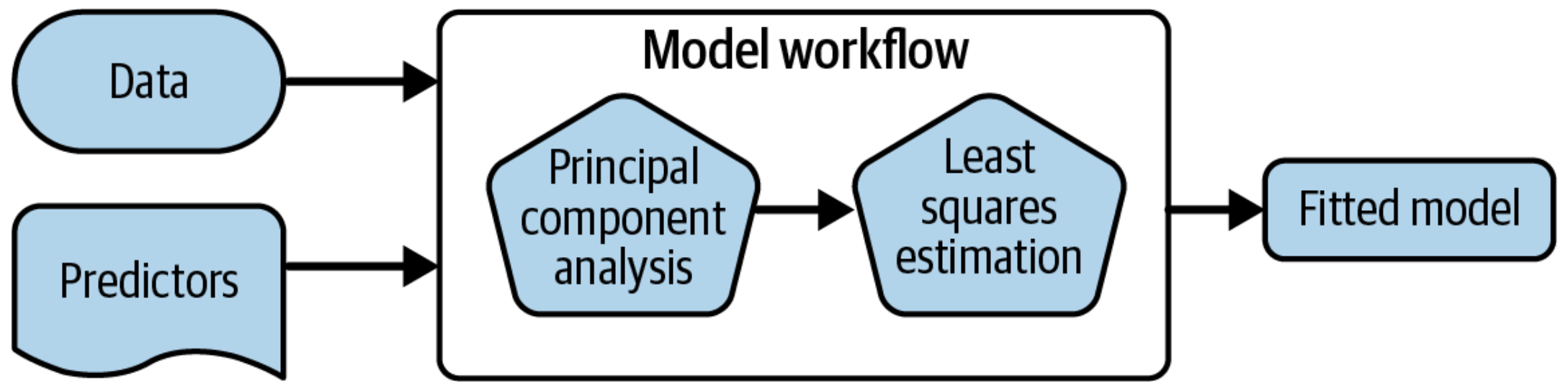
train_prediction <- xgboost_model_final |>
  # fit the model on all the training data
  fit(
    formula = nla_formula,
    data = train_processed
  ) |>
  # predict the sale prices for the training data
  predict(new_data = train_processed) |>
  bind_cols(
    nla_train |>
      mutate(.obs = log10(cyanophyta))
  )
xgboost_score_train <-
  train_prediction |>
  yardstick::metrics(.obs, .pred) |>
  mutate(.estimate = format(round(.estimate, 2), big.mark = ","))
knitr::kable(xgboost_score_train)

.metric	.estimator	.estimate
rmse	standard	0.79
rsq	standard	0.39
mae	standard	0.62

tidymodels - train evaluation

train_prediction |>
  ggplot(aes(.pred, .obs)) +
  geom_point() +
  geom_smooth(method = "lm")

tidymodels - test data

test_processed <- bake(nla_recipe, new_data = nla_test)

test_prediction <- xgboost_model_final |>
  # fit the model on all the training data
  fit(
    formula = nla_formula,
    data = train_processed
  ) |>
  # use the training model fit to predict the test data
  predict(new_data = test_processed) |>
  bind_cols(
    nla_test |>
      mutate(.obs = log10(cyanophyta))
  )

# measure the accuracy of our model using `yardstick`
xgboost_score <- test_prediction |>
  yardstick::metrics(.obs, .pred) |>
  mutate(.estimate = format(round(.estimate, 2), big.mark = ","))

knitr::kable(xgboost_score)

.metric	.estimator	.estimate
rmse	standard	0.79
rsq	standard	0.35
mae	standard	0.62

tidymodels - evaluation

cyanophyta_prediction_residual <- test_prediction |>
  arrange(.pred) %>%
  mutate(residual_pct = (.obs - .pred) / .pred) |>
  select(.pred, residual_pct)

cyanophyta_prediction_residual |>
  ggplot(aes(x = .pred, y = residual_pct)) +
  geom_point() +
  xlab("Predicted Cyanophyta") +
  ylab("Residual (%)")

tidymodels - test evaluation

test_prediction |>
  ggplot(aes(.pred, .obs)) +
  geom_point() +
  geom_smooth(method = "lm", colour = "black")

欢迎讨论！

苏命|https://drwater.net; https://drwater.net/team/ming-su/; Slides

mingsu@rcees.ac.cn;