数据可视化
《区域水环境污染数据分析实践》
Data analysis practice of regional water environment pollution

中国科学院大学资源与环境学院
中国科学院生态环境研究中心
2026-05-26
ggplot2::ggplot()

Data

Aesthetic Mapping(视觉映射):aes(.)
Geometries(几何图层):geom_*
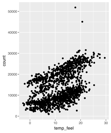
Visual Properties of Layers(图层属性)
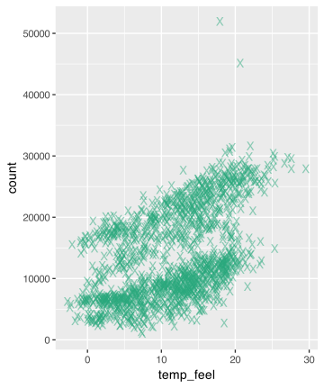
Setting vs Mapping of Visual Properties
ggplot(
  bikes,
  aes(x = temp_feel, y = count)
) +
  geom_point(
    color = "#28a87d",
    alpha = .5
  )
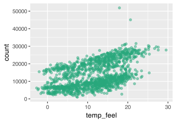
ggplot(
  bikes,
  aes(x = temp_feel, y = count)
) +
  geom_point(
    aes(color = season),
    alpha = .5
  )
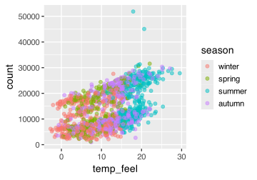
Mapping Expressions
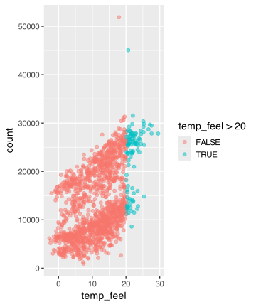
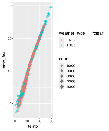
Filter Data
Filter Data
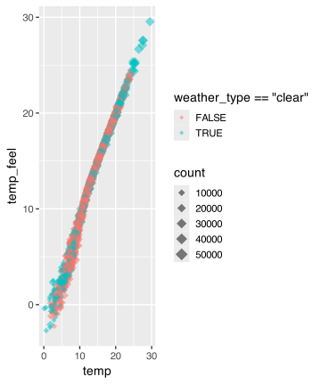
Local vs. Global(应用至当前图层或所有图层)
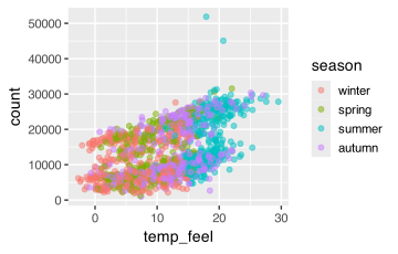
ggplot(
  bikes,
  aes(x = temp_feel, y = count)
) +
  geom_point(
    aes(color = season),
    alpha = .5
  )
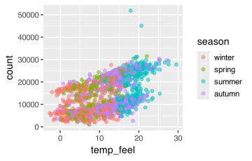
ggplot(
  bikes,
  aes(x = temp_feel, y = count, color = season)
) +
  geom_point(
    alpha = .5
  )
Adding More Layers
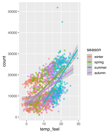
Global Color Encoding
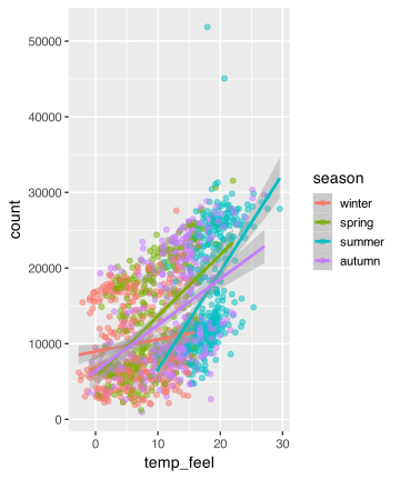
Local Color Encoding
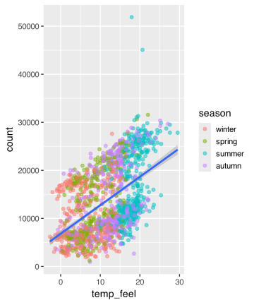
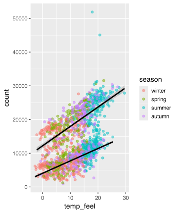
The `group` Aesthetic
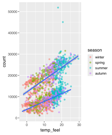
Set Both as Global Aesthetics
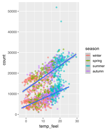
Overwrite Global Aesthetics
`stat_*()` and `geom_*()`
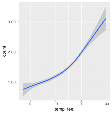
ggplot(bikes, aes(x = temp_feel, y = count)) +
  stat_smooth(geom = "smooth")
ggplot(bikes, aes(x = temp_feel, y = count)) +
  geom_smooth(stat = "smooth")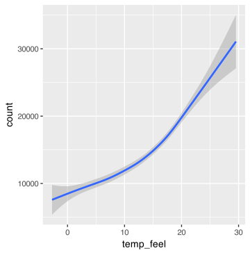
`stat_*()` and `geom_*()`
ggplot(bikes, aes(x = season)) +
  stat_count(geom = "bar")
ggplot(bikes, aes(x = season)) +
  geom_bar(stat = "count")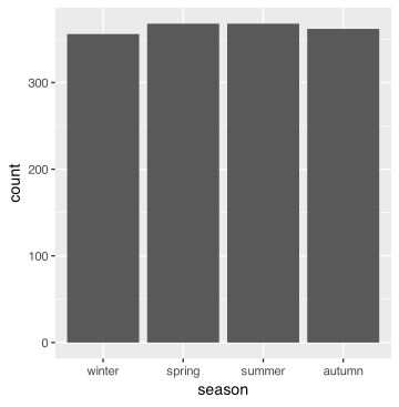
`stat_*()` and `geom_*()`
ggplot(bikes, aes(x = date, y = temp_feel)) +
  stat_identity(geom = "point")
ggplot(bikes, aes(x = date, y = temp_feel)) +
  geom_point(stat = "identity")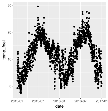
Statistical Summaries
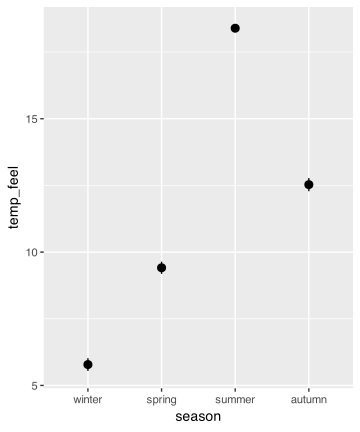
Statistical Summaries
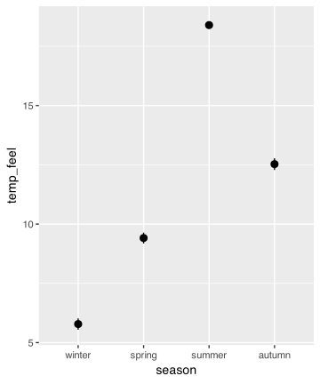
Statistical Summaries
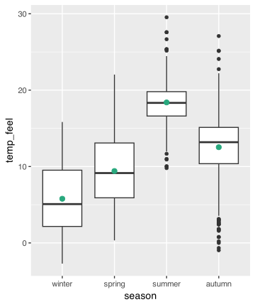
Statistical Summaries
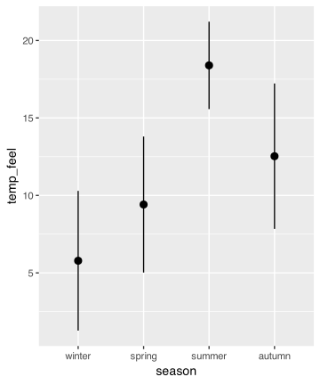
Extend a ggplot Object: Add Layers
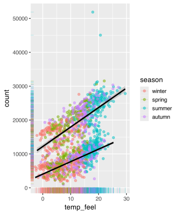
Remove a Layer from the Legend
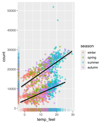
Extend a ggplot Object: Add Labels
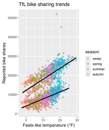
Extend a ggplot Object: Add Labels
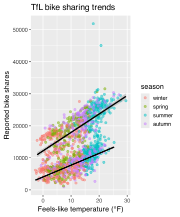
Extend a ggplot Object: Add Labels

Extend a ggplot Object: Add Labels
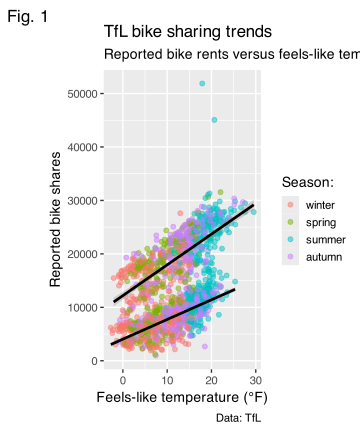
Extend a ggplot Object: Add Labels
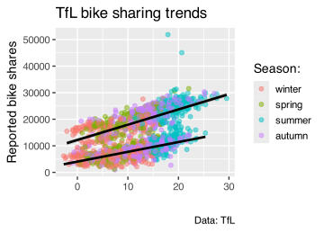
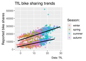
Extend a ggplot Object: Themes
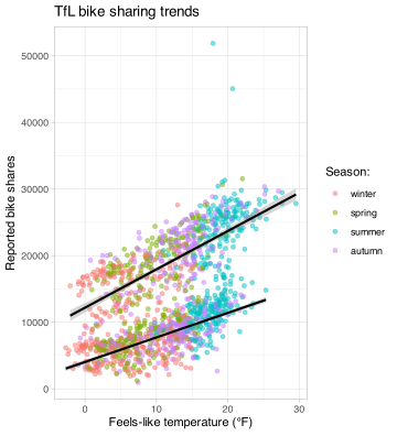
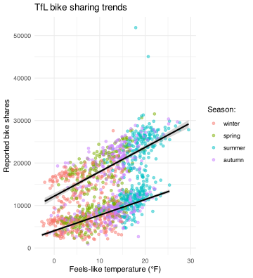
Change the Theme Base Settings
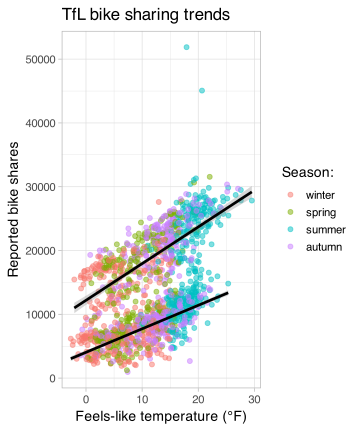
Set a Theme Globally
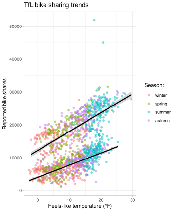
Change the Theme Base Settings
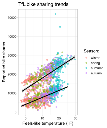
Overwrite Specific Theme Settings
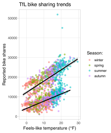
Overwrite Specific Theme Settings
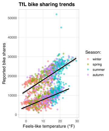
Overwrite Specific Theme Settings
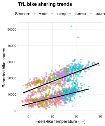
Overwrite Specific Theme Settings
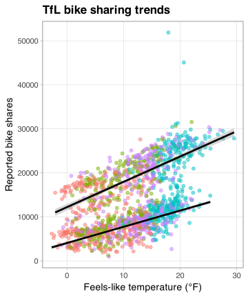
Overwrite Specific Theme Settings
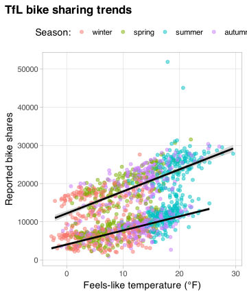
Overwrite Theme Settings Globally
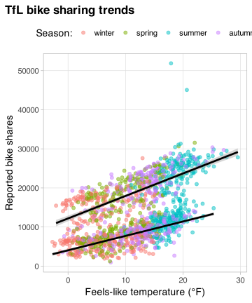


Setup
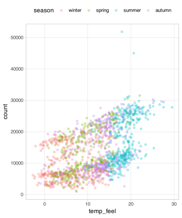
Wrapped Facets
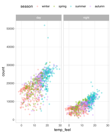
Wrapped Facets
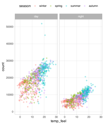
Facet Multiple Variables
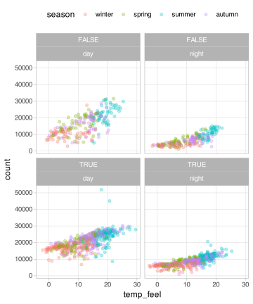
Facet Options: Cols + Rows
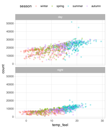
Facet Options: Free Scaling
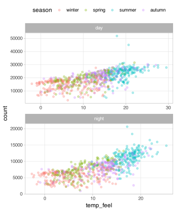
Facet Options: Free Scaling
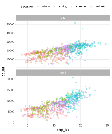
Facet Options: Switch Labels
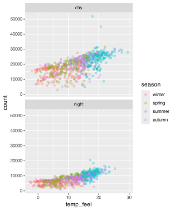
Gridded Facets
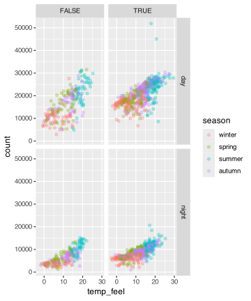
Gridded Facets
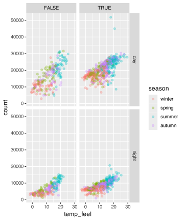
Facet Multiple Variables
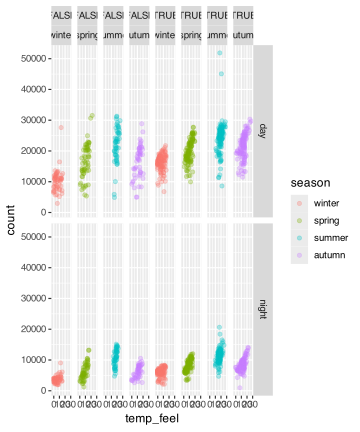
Facet Options: Free Scaling
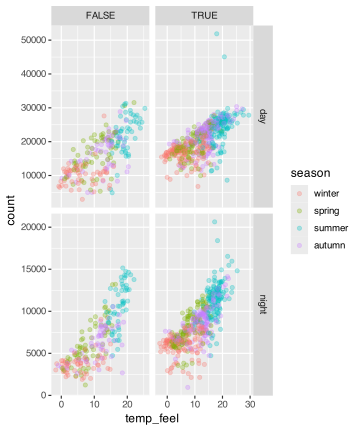
Facet Options: Switch Labels
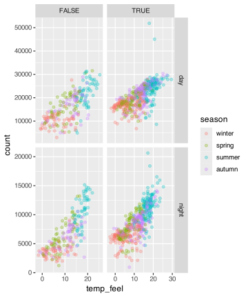
Facet Options: Proportional Spacing
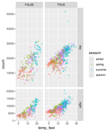
Facet Options: Proportional Spacing
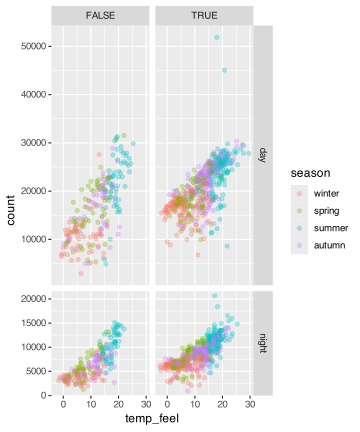
Diamonds Facet

Diamonds Facet

Diamonds Facet (Dark Theme Bonus)


Aesthetics + Scales
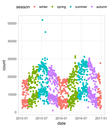
Aesthetics + Scales
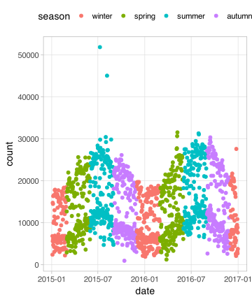
Scales
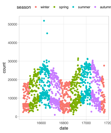
Scales

Scales
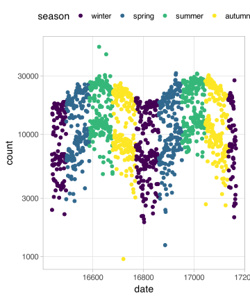
`scale_x|y_continuous`
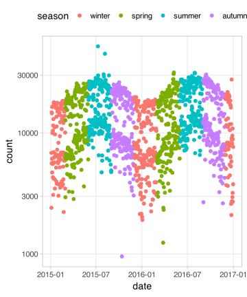
`scale_x|y_continuous`
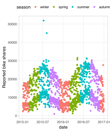
`scale_x|y_continuous`
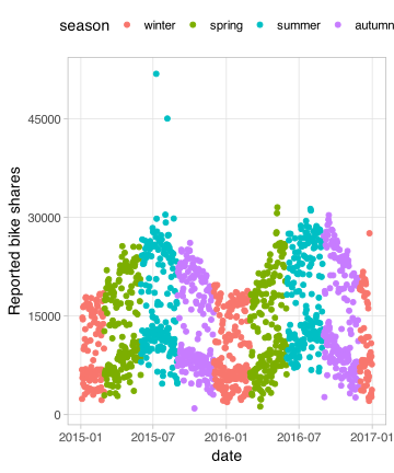
`scale_x|y_continuous`
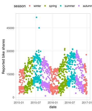
`scale_x|y_continuous`
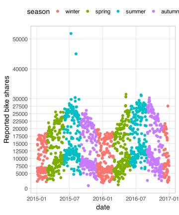
`scale_x|y_continuous`
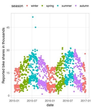
`scale_x|y_continuous`
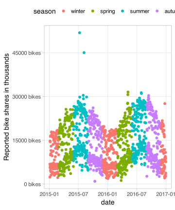
`scale_x|y_continuous`
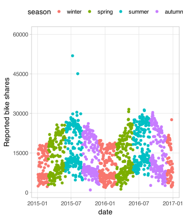
`scale_x|y_continuous`
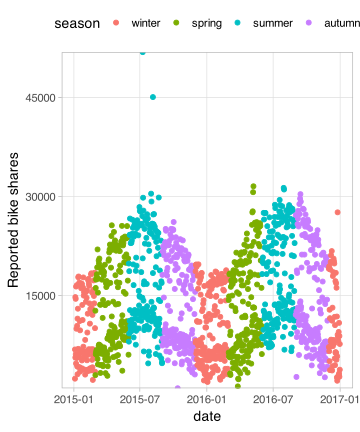
`scale_x|y_continuous`
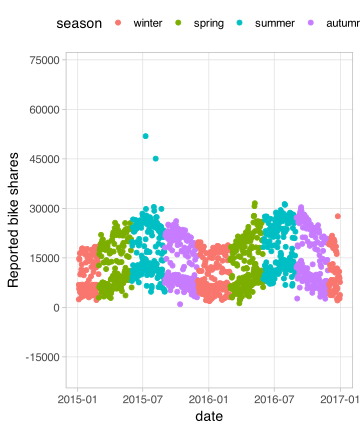
`scale_x|y_continuous`
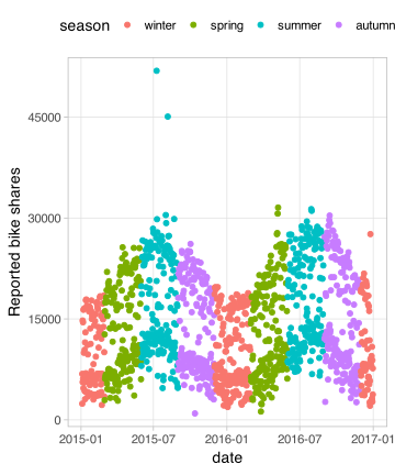
`scale_x|y_continuous`
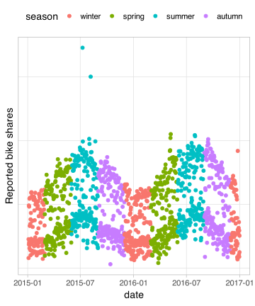
`scale_x|y_date`
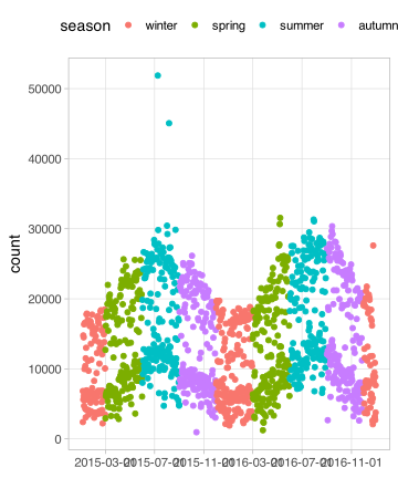
`scale_x|y_date`
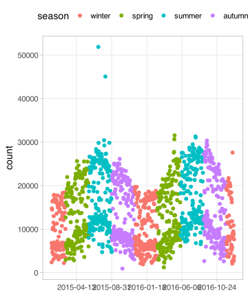
`scale_x|y_date` with `strftime()`
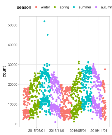
`scale_x|y_date` with `strftime()`
`scale_x|y_discrete`
`scale_x|y_discrete`
Discrete or Continuous?
Discrete or Continuous?
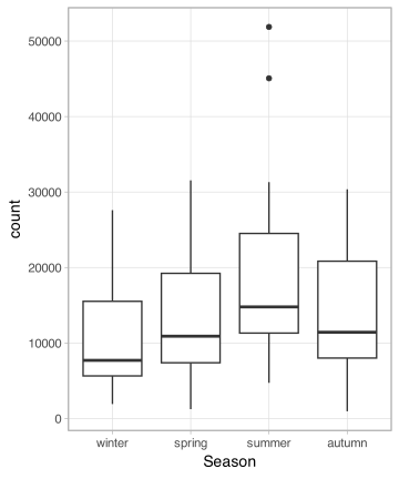
Discrete or Continuous?
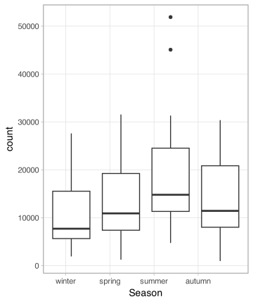
`scale_color|fill_discrete`

`scale_color|fill_discrete`

`scale_color|fill_discrete`

`scale_color|fill_discrete`

`scale_color|fill_manual`

Diamonds Facet

Diamonds Facet

Diamonds Facet

Diamonds Facet

Diamonds Facet

Diamonds Facet

Diamonds Facet

Cartesian Coordinate System
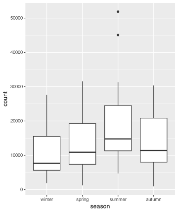
Cartesian Coordinate System
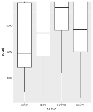
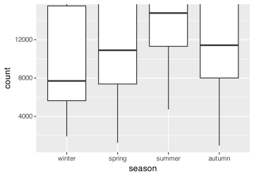
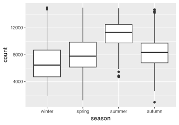
Changing Limits
ggplot(
  bikes,
  aes(x = season, y = count)
) +
  geom_boxplot() +
  coord_cartesian(
    ylim = c(NA, 15000)
  )
ggplot(
bikes,
aes(x = season, y = count)
) +
geom_boxplot() +
scale_y_continuous(
limits = c(NA, 15000)
)
Clipping
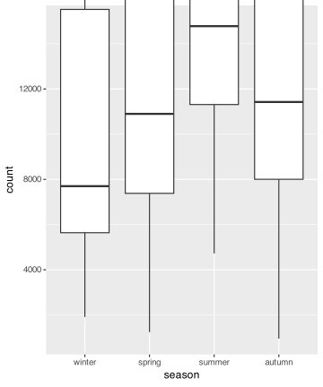
Clipping
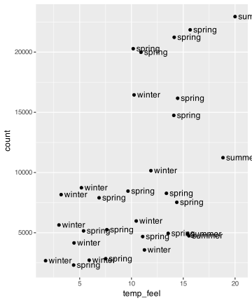
… or better use {ggrepel}
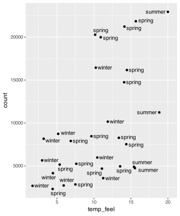
Remove All Padding
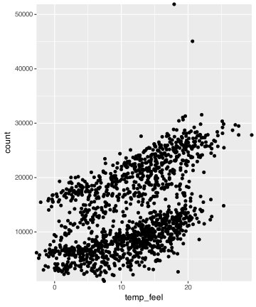
Fixed Coordinate System
ggplot(
  bikes,
  aes(x = temp_feel, y = temp)
) +
  geom_point() +
  coord_fixed()
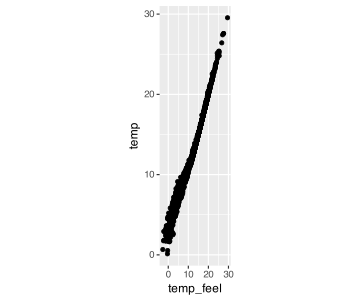
ggplot(
  bikes,
  aes(x = temp_feel, y = temp)
) +
  geom_point() +
  coord_fixed(ratio = 4)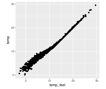
Flipped Coordinate System
ggplot(
  bikes,
  aes(x = weather_type)
) +
  geom_bar() +
  coord_cartesian()
ggplot(
  bikes,
  aes(x = weather_type)
) +
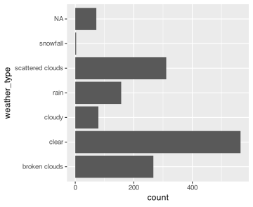
  geom_bar() +
  coord_flip()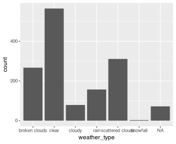
Flipped Coordinate System
ggplot(
  bikes,
  aes(y = weather_type)
) +
  geom_bar() +
  coord_cartesian()
ggplot(
  bikes,
  aes(x = weather_type)
) +
  geom_bar() +
  coord_flip()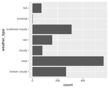
Reminder: Sort Your Bars!

Reminder: Sort Your Bars!

Circular Corrdinate System
ggplot(
  filter(bikes, !is.na(weather_type)),
  aes(x = weather_type, fill = weather_type)
) +
  geom_bar() +
  coord_polar()
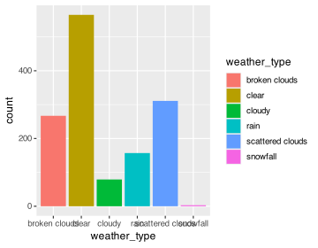
ggplot(
  filter(bikes, !is.na(weather_type)),
  aes(x = weather_type, fill = weather_type)
) +
  geom_bar() +
  coord_cartesian()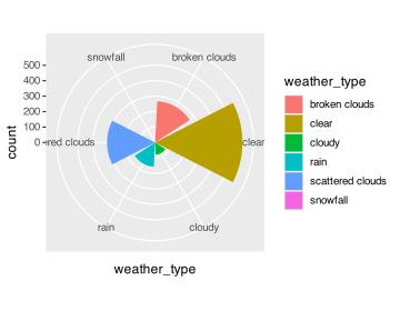
Circular Cordinate System
ggplot(
  filter(bikes, !is.na(weather_type)),
  aes(x = fct_infreq(weather_type), fill = weather_type)
) +
  geom_bar(width = 1) +
  coord_polar()
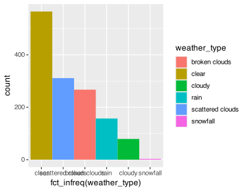
ggplot(
  filter(bikes, !is.na(weather_type)),
  aes(x = fct_infreq(weather_type), fill = weather_type)
) +
  geom_bar(width = 1) +
  coord_cartesian()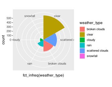
Circular Corrdinate System
ggplot(
  filter(bikes, !is.na(weather_type)),
  aes(x = fct_infreq(weather_type), fill = weather_type)
) +
  geom_bar() +
  coord_polar(theta = "x")
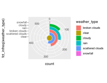
ggplot(
  filter(bikes, !is.na(weather_type)),
  aes(x = fct_infreq(weather_type), fill = weather_type)
) +
  geom_bar() +
  coord_polar(theta = "y")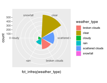
Circular Corrdinate System
ggplot(
  filter(bikes, !is.na(weather_type)),
  aes(x = 1, fill = weather_type)
) +
  geom_bar(position = "stack") +
  coord_polar(theta = "y")
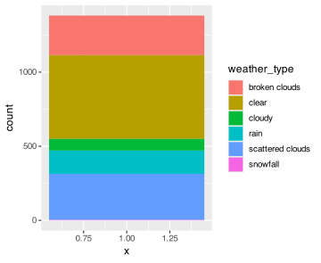
ggplot(
  filter(bikes, !is.na(weather_type)),
  aes(x = 1, fill = weather_type)
) +
  geom_bar(position = "stack") +
  coord_cartesian()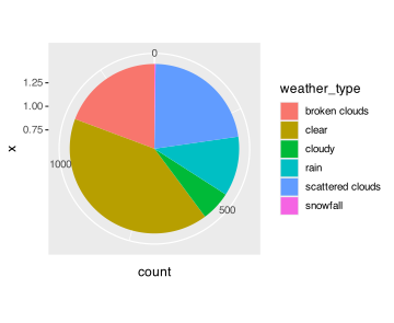
Circular Corrdinate System
ggplot(
  filter(bikes, !is.na(weather_type)),
  aes(x = 1, fill = fct_rev(fct_infreq(weather_type)))
) +
  geom_bar(position = "stack") +
  coord_polar(theta = "y") +
  scale_fill_discrete(name = NULL)
ggplot(
  filter(bikes, !is.na(weather_type)),
  aes(x = 1, fill = fct_rev(fct_infreq(weather_type)))
) +
  geom_bar(position = "stack") +
  coord_cartesian() +
  scale_fill_discrete(name = NULL)

Transform a Coordinate System
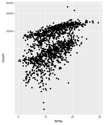
Transform a Coordinate System
ggplot(
  bikes,
  aes(x = temp, y = count, group = day_night)
) +
  geom_point() +
  geom_smooth(method = "lm") +
  coord_trans(y = "log10")
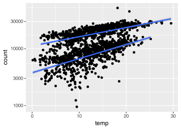
ggplot(
  bikes,
  aes(x = temp, y = count, group = day_night)
) +
  geom_point() +
  geom_smooth(method = "lm") +
  scale_y_log10()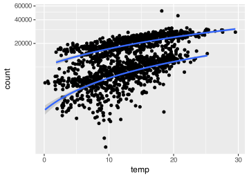

theme_std <- theme_set(theme_minimal(base_size = 18))
theme_update(
  # text = element_text(family = "Pally"),
  panel.grid = element_blank(),
  axis.text = element_text(color = "grey50", size = 12),
  axis.title = element_text(color = "grey40", face = "bold"),
  axis.title.x = element_text(margin = margin(t = 12)),
  axis.title.y = element_text(margin = margin(r = 12)),
  axis.line = element_line(color = "grey80", size = .4),
  legend.text = element_text(color = "grey50", size = 12),
  plot.tag = element_text(size = 40, margin = margin(b = 15)),
  plot.background = element_rect(fill = "white", color = "white")
)

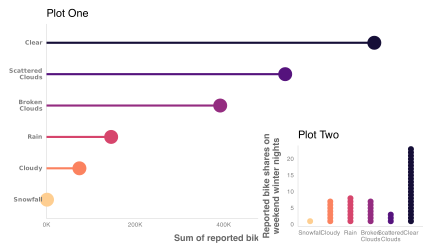
bikes_sorted <-
  bikes %>%
  filter(!is.na(weather_type)) %>%
  group_by(weather_type) %>%
  mutate(sum = sum(count)) %>%
  ungroup() %>%
  mutate(
    weather_type = forcats::fct_reorder(
      str_to_title(str_wrap(weather_type, 5)),
      sum
    )
  )

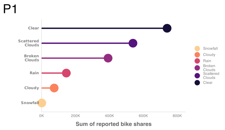
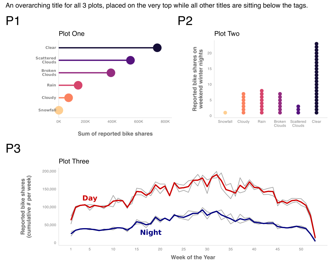
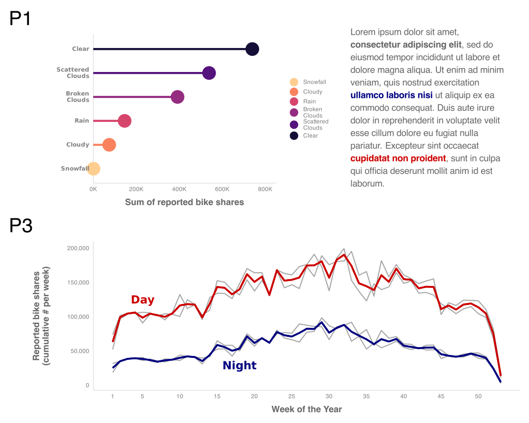
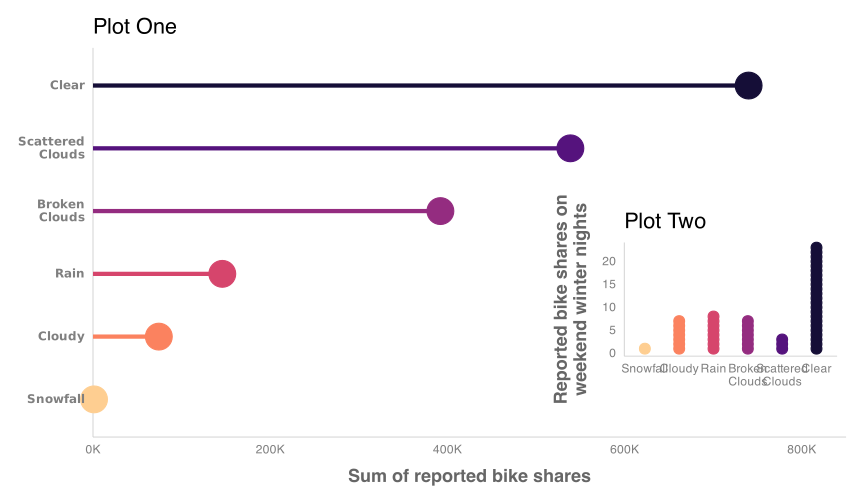
p1 <- ggplot(
  bikes_sorted,
  aes(x = weather_type, y = count, color = weather_type)
) +
  geom_hline(yintercept = 0, color = "grey80", size = .4) +
  stat_summary(
    geom = "point",
    fun = "sum",
    size = 12
  ) +
  stat_summary(
    geom = "linerange",
    ymin = 0,
    fun.max = function(y) sum(y),
    size = 2,
    show.legend = FALSE
  ) +
  coord_flip(ylim = c(0, NA), clip = "off") +
  scale_y_continuous(
    expand = c(0, 0),
    limits = c(0, 8500000),
    labels = scales::comma_format(scale = .0001, suffix = "K")
  ) +
  scale_color_viridis_d(
    option = "magma",
    direction = -1,
    begin = .1,
    end = .9,
    name = NULL,
    guide = guide_legend(override.aes = list(size = 7))
  ) +
  labs(
    x = NULL,
    y = "Sum of reported bike shares",
    tag = "P1",
  ) +
  theme(
    axis.line.y = element_blank(),
    axis.text.y = element_text(
      family = "Pally",
      color = "grey50",
      face = "bold",
      margin = margin(r = 15),
      lineheight = .9
    )
  )

p1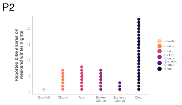
p2 <- bikes_sorted %>%
  filter(season == "winter", is_weekend == TRUE, day_night == "night") %>%
  group_by(weather_type, .drop = FALSE) %>%
  mutate(id = row_number()) %>%
  ggplot(
    aes(x = weather_type, y = id, color = weather_type)
  ) +
  geom_point(size = 4.5) +
  scale_color_viridis_d(
    option = "magma",
    direction = -1,
    begin = .1,
    end = .9,
    name = NULL,
    guide = guide_legend(override.aes = list(size = 7))
  ) +
  labs(
    x = NULL,
    y = "Reported bike shares on\nweekend winter nights",
    tag = "P2",
  ) +
  coord_cartesian(ylim = c(.5, NA), clip = "off")

p2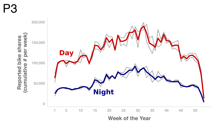
my_colors <- c("#cc0000", "#000080")

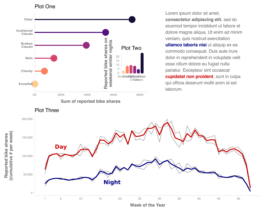
p3 <- bikes %>%
  group_by(week = lubridate::week(date), day_night, year) %>%
  summarize(count = sum(count)) %>%
  group_by(week, day_night) %>%
  mutate(avg = mean(count)) %>%
  ggplot(aes(x = week, y = count, group = interaction(day_night, year))) +
  geom_line(color = "grey65", size = 1) +
  geom_line(aes(y = avg, color = day_night), stat = "unique", size = 1.7) +
  annotate(
    geom = "text",
    label = c("Day", "Night"),
    color = my_colors,
    x = c(5, 18),
    y = c(125000, 29000),
    size = 8,
    fontface = "bold",
    family = "Pally"
  ) +
  scale_x_continuous(breaks = c(1, 1:10 * 5)) +
  scale_y_continuous(labels = scales::comma_format()) +
  scale_color_manual(values = my_colors, guide = "none") +
  labs(
    x = "Week of the Year",
    y = "Reported bike shares\n(cumulative # per week)",
    tag = "P3",
  )

p3
{patchwork}
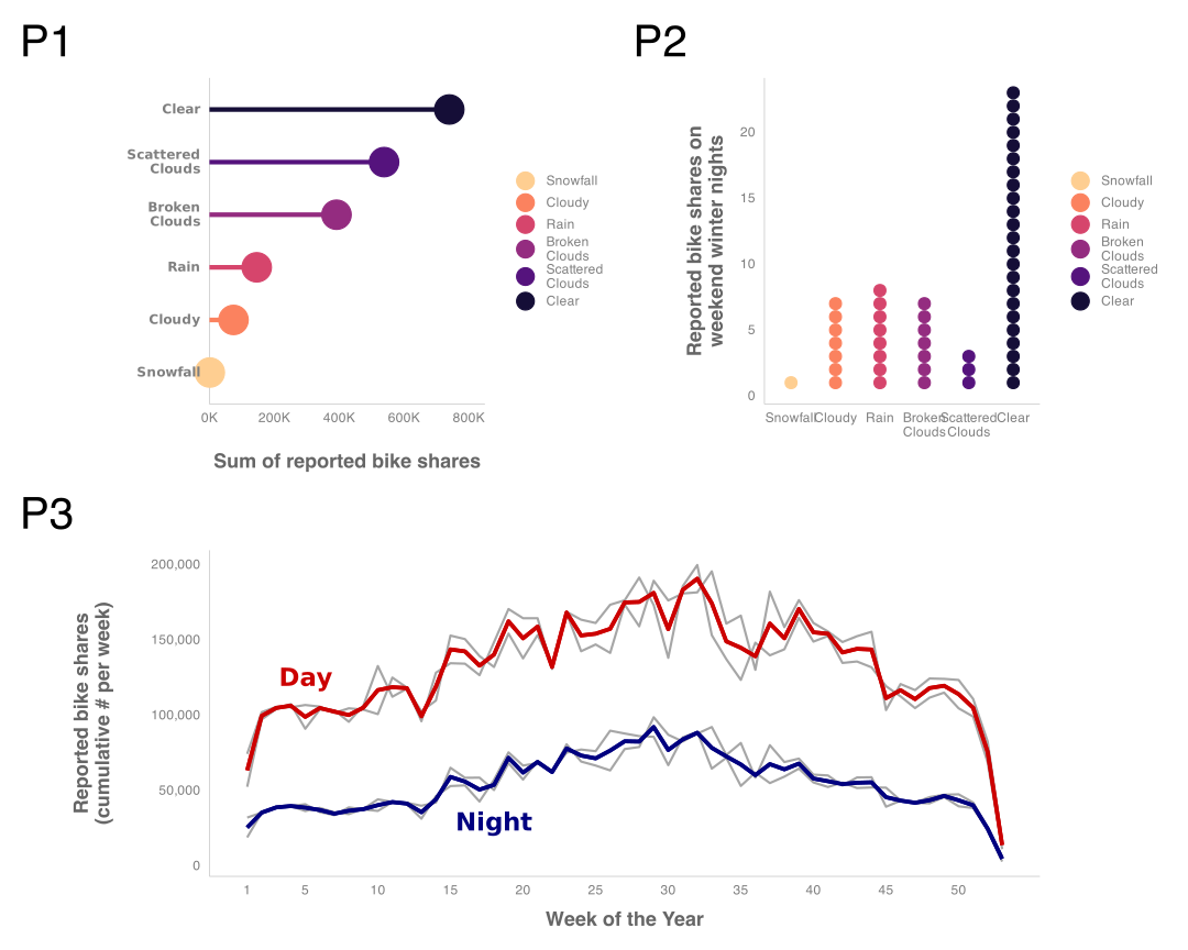
“Collect Guides”
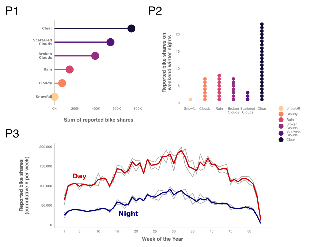
Apply Theming
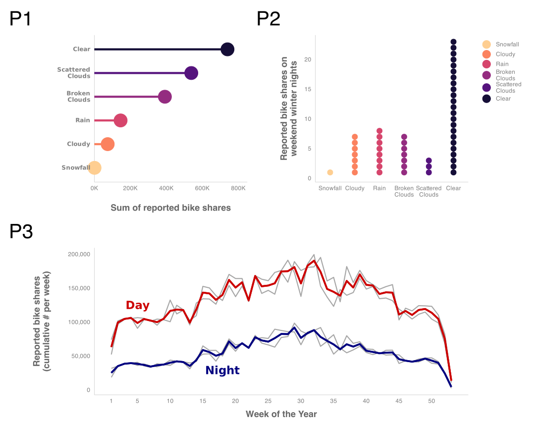
Apply Theming
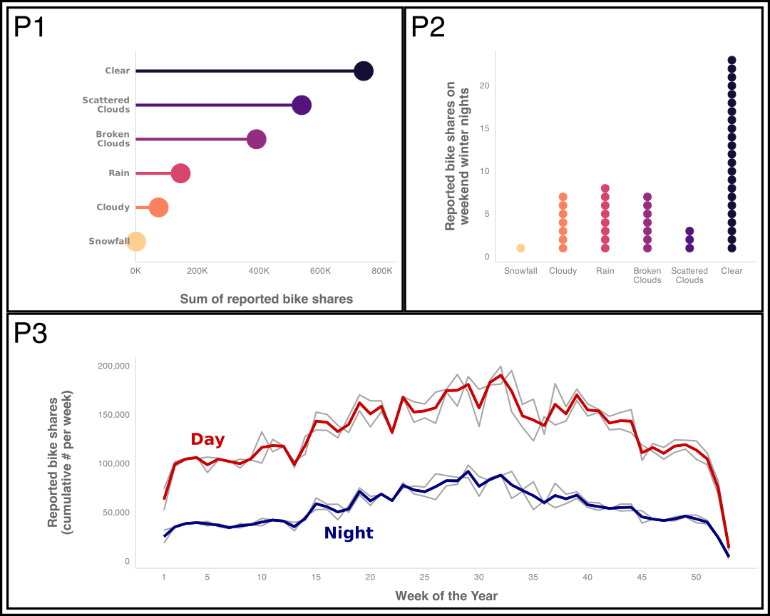
Adjust Widths and Heights
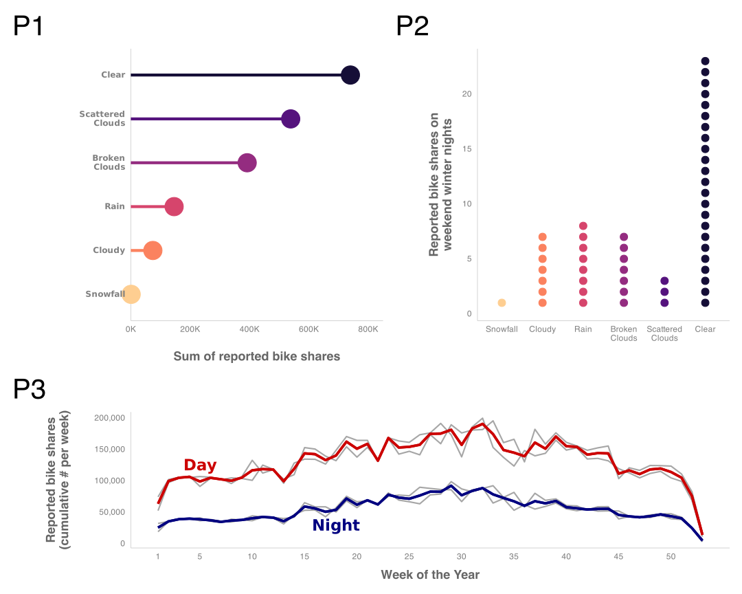
Use A Custom Layout
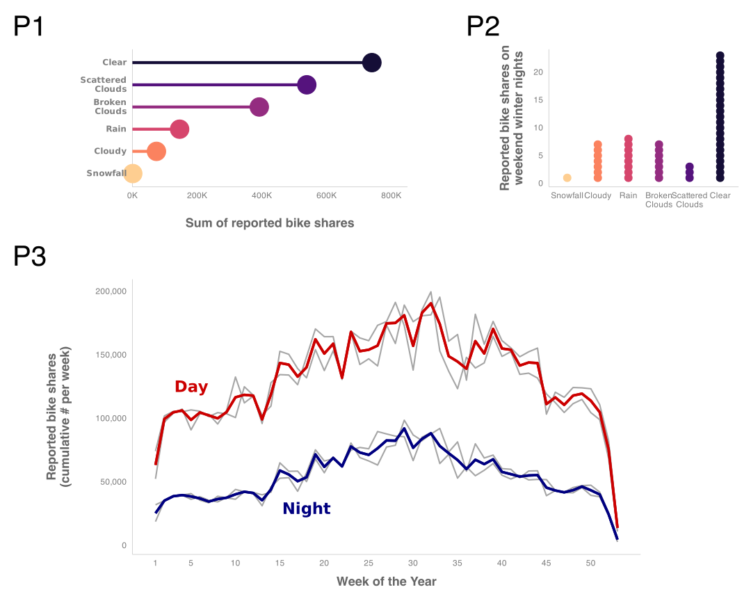
Add Labels
Add Text
text <- tibble::tibble(
  x = 0,
  y = 0,
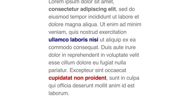
  label = "Lorem ipsum dolor sit amet, **consectetur adipiscing elit**, sed do eiusmod tempor incididunt ut labore et dolore magna aliqua. Ut enim ad minim veniam, quis nostrud exercitation <b style='color:#000080;'>ullamco laboris nisi</b> ut aliquip ex ea commodo consequat. Duis aute irure dolor in reprehenderit in voluptate velit esse cillum dolore eu fugiat nulla pariatur. Excepteur sint occaecat <b style='color:#cc0000;'>cupidatat non proident</b>, sunt in culpa qui officia deserunt mollit anim id est laborum."
)
pt <- ggplot(text, aes(x = x, y = y)) +
  ggtext::geom_textbox(
    aes(label = label),
    box.color = NA,
    width = unit(23, "lines"),
    color = "grey40",
    size = 6.5,
    lineheight = 1.4
  ) +
  coord_cartesian(expand = FALSE, clip = "off") +
  theme_void()
pt
Add Text
Add Inset Plots
Add Inset Plots
Add Inset Plots
效果
练习
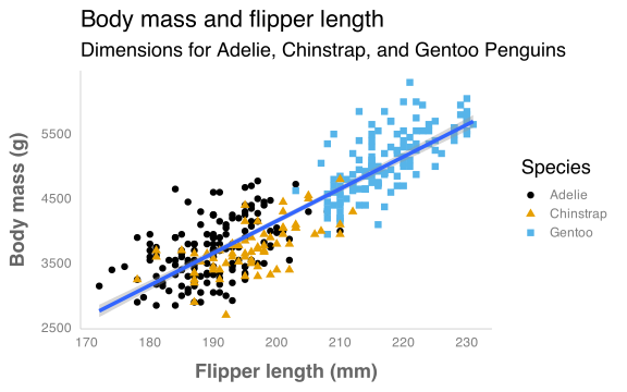
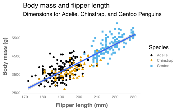
p <- ggplot(
  data = penguins,
  mapping = aes(x = flipper_length_mm, y = body_mass_g)
) +
  geom_point(aes(color = species, shape = species)) +
  geom_smooth(method = "lm") +
  labs(
    title = "Body mass and flipper length",
    subtitle = "Dimensions for Adelie, Chinstrap, and Gentoo Penguins",
    x = "Flipper length (mm)",
    y = "Body mass (g)",
    color = "Species",
    shape = "Species"
  ) +
  scale_color_colorblind()